Volume Slices and Isosurfaces

Table of Contents, Get code for this tutorial

Note: You can execute the code from this tutorial by highlighting them, right-clicking, and selecting "Evaluate Selection" (or hit F9).

This is based on a video tutorial on Doug's Video Tutorial blog.

In this section, you'll learn how you can visualize volumetric data by slicing into the data and creating isosurfaces. Specifically, you will learn at how to visualize scalar fields. Scalar fields contain scalar information for every point in space. For example, temperature inside a room is a scalar field. In the next section, you will examine techniques for visualizing vector fields.

Understanding Volumetric Data
Slices through Volumetric Data
Contour Slices
Isosurfaces
3D Animation

Understanding Volumetric Data

Let's start with a simple example to understand what volumetric data is and how it's represented in MATLAB.

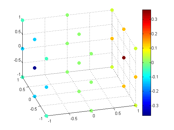
We'll define volumetric data by assigning a value at every 3D grid point. Let's look at a simple, coarse-grained example

[x, y, z] = meshgrid([-1 0 1]);
v = x .* exp(-x.^2 - y.^2 - z.^2);

We'll use scatter3 to visualize the values at each grid point.

scatter3(x(:), y(:), z(:), 72, v(:), 'filled');
view(-15, 35);
colorbar;

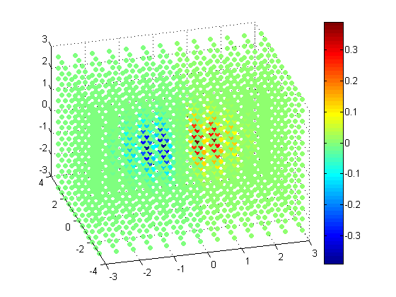
Let's look at a larger data set by increasing the resolution.

[x,y,z] = meshgrid(-3:0.5:3);
v = x.*exp(-x.^2 - y.^2 - z.^2);
scatter3(x(:), y(:), z(:), 30, v(:), 'filled');
view(-15, 35);
colorbar;

Slices through Volumetric Data

As you can see, the higher the resolution gets, the harder it becomes to visualize. One way of understanding volumetric data is to take a slice out of it.

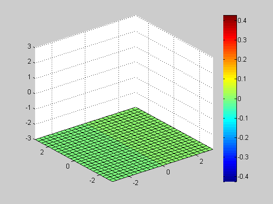
Slice along Z = 0

% Even higher resolution
[x, y, z] = meshgrid(-3:0.25:3);
v = x.*exp(-x.^2 - y.^2 - z.^2);

slice(x, y, z, v, [], [], 0);
colorbar;

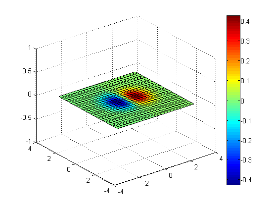
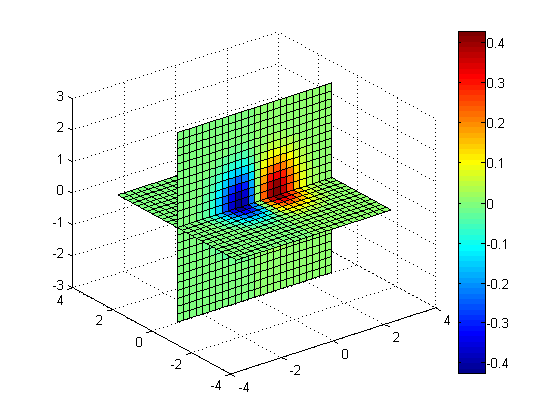
Slices along Y = 0 and Z = 0

slice(x, y, z, v, [], 0, 0);
colorbar;

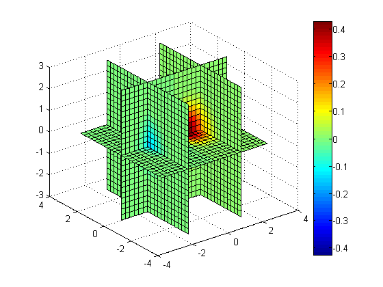
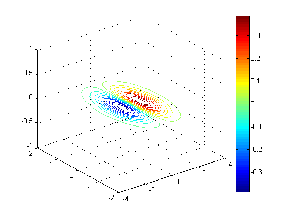
Slices along X = 1.5, X = -1.5, Y = 0, Z = 0

slice(x, y, z, v, [1.5 -1.5], 0, 0);
colorbar;

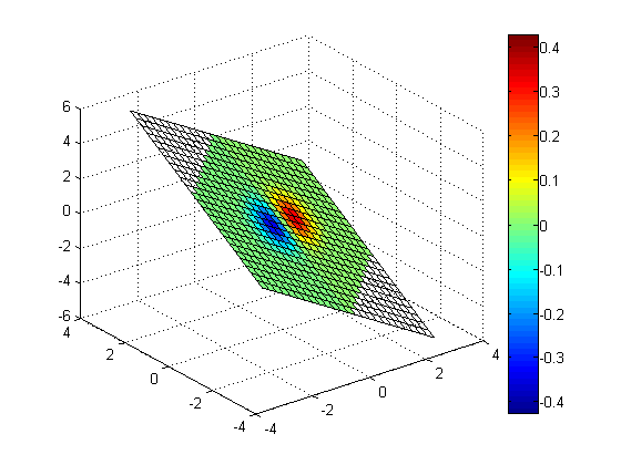
Slice along Z = -X + Y

[xs, ys] = meshgrid(-3:0.25:3);
zs = -xs + ys;
slice(x, y, z, v, xs, ys, zs);
colorbar;

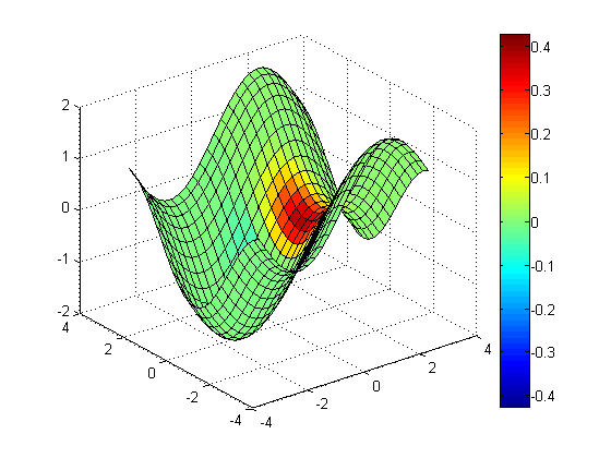
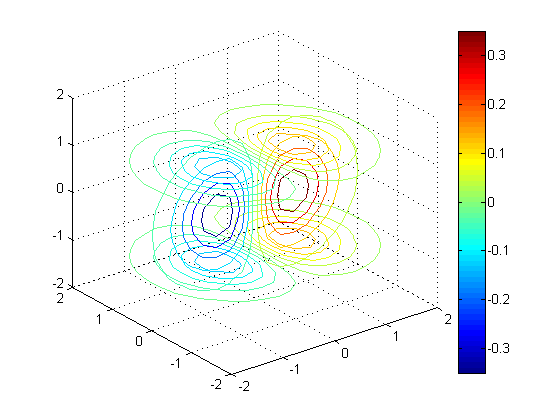
Slice along non-planar surface, Z = sin(X) - cos(Y)

zs = sin(xs) - cos(ys);
slice(x, y, z, v, xs, ys, zs);
colorbar;

Contour Slices

You can create contour slices using contourslice.

Contour slice along Z = 0

clf
contourslice(x, y, z, v, [], [], 0, 20);     % 20 contour lines
view(3); grid on;
colorbar;

Contour slice along Y = 0, Z = -1, Z = 1

clf;
contourslice(x, y, z, v, [], 0, [-1 1], 10); % 10 contour lines
view(3); grid on;
colorbar;

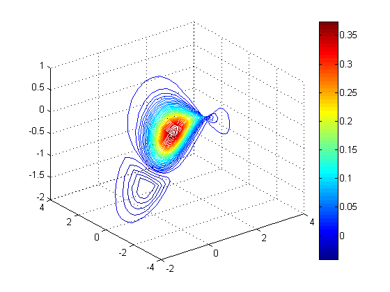
Contour slice along Z = sin(X) - cos(Y/2)

clf;
zs = sin(xs) - cos(ys/2);
contourslice(x, y, z, v, xs, ys, zs, 50);    % 50 contour lines
view(3); grid on;
colorbar;

Isosurfaces

In contrast to making slices (whether they're flat planes or nonlinear), a different way of exploring volumetric data is to view the "boundaries". If you connect all the points with the same value, you get an isosurface

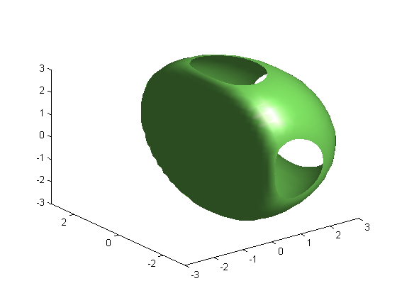
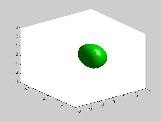
Isosurface where V = 1e-5

clf;
isosurface(x, y, z, v, 1e-5);
axis([-3 3 -3 3 -3 3]);

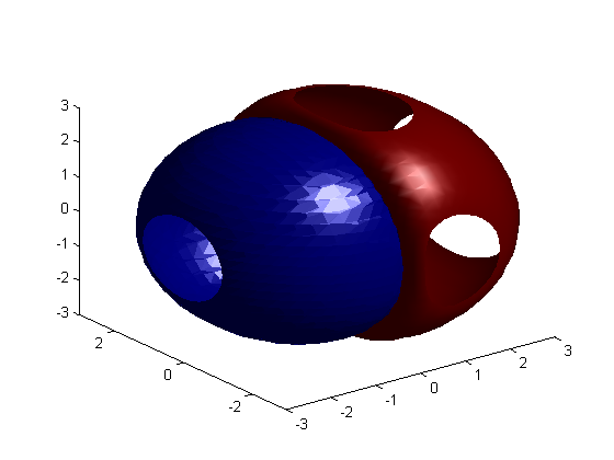
Isosurface where V = 1e-5 and V = -1e-4

clf;
isosurface(x, y, z, v, 1e-5);
isosurface(x, y, z, v, -1e-4);
axis([-3 3 -3 3 -3 3]);

3D Animation

Let's put these visualization commands in a FOR loop to animate.

Isosurface

clf;
vals = logspace(-1, -5, 25);  % 20 points from 1e-1 down to 1e-5
h = patch(isosurface(x, y, z, v, vals(1)), ...
   'facecolor', 'g', 'edgecolor', 'none');
axis([-3 3 -3 3 -3 3]);
camlight; lighting phong
for id = vals
   [faces, vertices] = isosurface(x, y, z, v, id);
   set(h, 'Faces', faces, 'Vertices', vertices);
   pause(0.1);
end

close;

Slice

clf;
vals = -3:0.25:3;
h= slice(x, y, z, v, [], [], vals(1));
axis([-3 3 -3 3 -3 3]);
colorbar;
for id = vals
   delete(h);
   h= slice(x, y, z, v, [], [], id);
   axis([-3 3 -3 3 -3 3]);
   colorbar;
   pause(0.1);
end

close;

Table of Contents