9.29 MEA Network Topology
Characterization:
small-world and scale-free networks
Project Report
Ulf Knoblich and Ji-Jon Sit
Abstract
Our project attempts to determine the characteristics of the neuronal network underlying a multi-electrode array (MEA), which records spike firing by neurons in the vicinity of each electrode. Spike timings were obtained from the noisy data by performing some preprocessing, and then the spike times were analyzed using two different methods to generate a directed graph representing the connectivity in the neuronal network. Simplifying assumptions are made by having to lump the behavior of possibly many neurons into a single electrode channel. However, the measurements of average path length L and clustering coefficient C as defined in the literature still turn out to be robust and largely invariant to our choice of method and parameters used in generating the graph. This lends some confidence to the reliability and reproducibility of the results. Measurements of degree distribution P(k) from the graph, however, turn out to be inconclusive primarily due to the limited size of the dataset.
Introduction
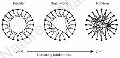
In recent years, with the abundance of storage and availability of information, the characterization of networks has become a focus of the scientific community again, picking up and enhancing the work of Erdös, who modeled large natural networks as random. Watts and Strogatz examined so-called small-world networks, which successfully model a large variety of social and biological networks such as actor collaborations, friend networks, the C. elegans neural network etc.
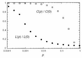
They systematically investigated the transition from regular networks to random networks by rewiring edges in a regular network with increasing probability, as illustrated below [taken from Watts and Strogatz]. The two network characteristics they used are the average path length L, which defines the average number of edges between any two nodes in the network, and the average cliquishness C, which is a measure for how many neighbors of a node are neighbors of each other. It turns out that the rewiring of only very few edges drastically decreases C while L stays almost unaffected. As the plot on the right shows, there is a large regime where L is close to random networks whereas C is close to the value for regular networks. The authors label this configuration of L and C as small-world characteristics.
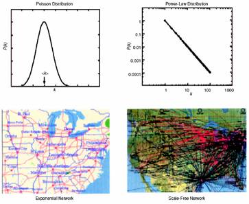
Barabasi and Albert picked up the notion of small-world networks and added the scale-free property to the characteristics under investigation. The scale-free property states that the degree distribution of nodes in the nework is a power-law instead of a Poisson distribution, as would be expected for random networks. The degree distribution is the distribution of the number of edges for each node. In their paper they showed that several of the networks investigated by Watts and Strogatz actually exhibit the scale-free property, such as the actor collaboration graph, the US power grid, a citation graph, the Internet etc. They explain and simulate the emergence of this property by two assumptions. First, nodes are actually added to the network sequentially. This makes sense in the above mentioned cases where new computers are added to the Internet over time.The second assumption is that a new node is more likely to be connected to a node which is already well-connected,i.e. has a high degree. This is the well-known ‘rich-get-richer’ phenomenon. The figure below shows two examples for a Poisson and a power law distributionnetwork [taken from Barabasi and Albert].
Subsequently, it was shown that these properties have important implication for dynamic properties of networks such as the speed of spread of a disease in social networks or the ability for synchronization. As the topic of neural network dynamics is still unresolved, our goal was to investigate whether data from MEA recordings actually exhibit these properties (small-world and scale-free) in order to generate more data about structural properties of thee networks.
Methods
Filtering of Raw Data
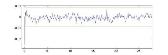
The first thing we needed to do was clean up the raw voltage waveforms. There was a considerable amount of 60Hz noise in the original signal s(t), as the graph below will show:
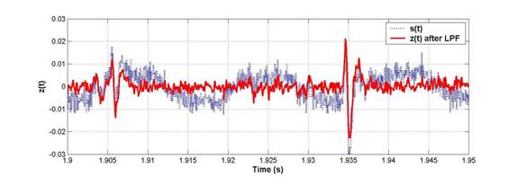
To extract clean spikes as shown by z(t) out of the 60Hz noise, we performed 2 filtering steps: first, a series of 3rd-order notch filters were applied, and second, a 2nd-order low-pass filter with a 5kHz roll-off was used on the notched spectrum.
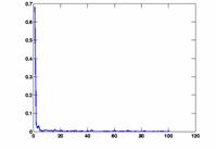
3rd-order selective notch filtering: To start, a FFT was taken (shown below), and any spikes in the FFT above a value of 11 (set arbitrarily) would be notched out.
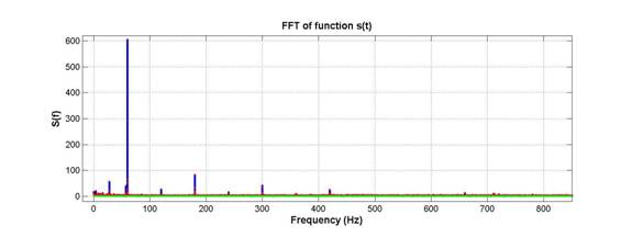
As seen above, the 60Hz and harmonics are huge. The notch filter we used was designed in the spirit of a 3rd order Butterworth filter, for which a low-pass version is given by:
![]()
The reason for this choice was to avoid brick-wall drop-offs in the frequency spectrum, which would happen if the offending peaks were just zeroed out. We figured that brick-wall discontinuities in the spectrum would be undesirable because they introduce artifacts in the time-domain that will ring on for infinite time.
The actual notch filter was implemented as a 1/(1+x(f)3) attenuation where x(f) = the size of the spike at its peak, but dropping with a 1/f roll-off as f moves away from the peak. Hence the notch filter is sharp (3rd-order) but not discontinuous. The MATLAB code to do this is notch.m.
The frequency spectrum after notch filtering is shown below. A fuzz in the spectrum above 5kHz was noticed. This motivated the need for a 5kHz low-pass filter.
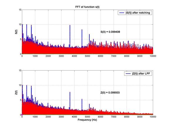
2nd-order 5kHz low-pass filtering: As shown above, after the low pass filter was applied, the spectrum looks considerably cleaner at high frequencies. This had a very significant effect in the time domain, as shown below:
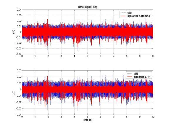
The level of the noise is much reduced, and hence the spike-to-noise discrimination was highly improved by the LPF. Zooming in to a plot of s(t) and z(t) near 2s, we can see that both small and large spikes are picked up when we apply a 5s threshold to distinguish spikes from the noise.
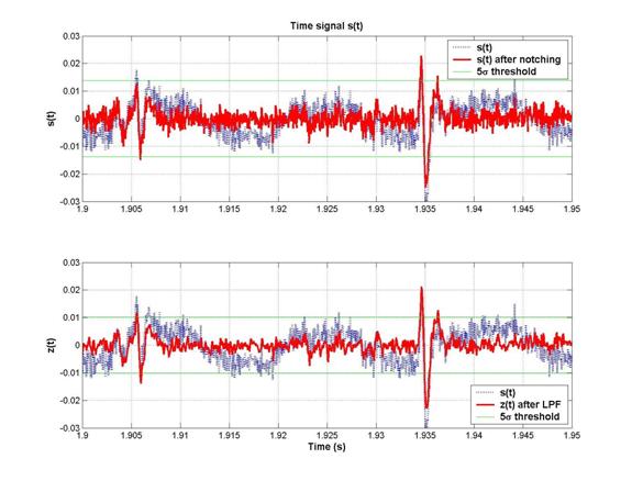
In conclusion, we can observe that spike-detection would have been almost impossible without the notching, and much less reliable without the low-pass filtering. The code to apply this filtering on all the 64 channels at once is processdata.m.
Spike Timing Extraction
Now that we have clean voltage waveforms, we determined the exact time of a spike by looking within 0.4ms windows for a voltage excursion that exceeded 5s. These spike times were saved into a matrix. We also ignored large glitches larger than 7s at the beginning of the data, as we observed in some channels. We did not consider these glitches as spikes:
The final spike times extracted from the 64 channels are shown below:
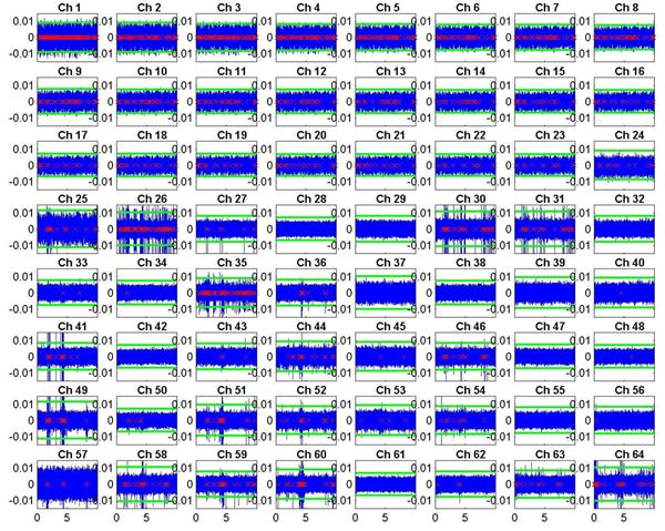
The raw (and filtered) voltage waveform is shown in blue. The time of extracted spikes are shown as red crosses along the x-axis. The green lines show the 5s threshold that determines the presence of a spike. Two observations should be made about this data:
1) The
first 24 channels turned out to be almost exact replicas of each other, just
scaled by some constant factor with varying amounts of additional noise. Hence
we ignored the first 24 channels, as they were deemed to contain no useful
information.
2) Of the remaining 40 channels (25-64), only about half of them show significant levels of spiking. Hence the final graphs will omit most of the blank channels as well.
The scripts which extract and plot these spikes are listed: get_sp.m, s4std.m, s5std.m, plot_sp.m, plot_spALL.m.
Edge determination
It is unclear exactly what sort of method should be used to infer connectivity between the channels, based merely on the spike timings. Thus we wanted to test more than one plausible method for determining an edge (i.e. a directed connection) between each node (i.e. each channel).
Delay histogram
method of edge determination
A very intuitive method to infer connections between nodes is to determine whether there is a relationship beween a spike on one node and the next spike on another node. If there is a connection between the two nodes, the probability that spiking at the first node triggers spiking at the second node should be high, which will produce a peak in the distribution of delay times between the a spike on one channel and the following spike on the other channel.
We calculated the delay histogram for every channel pair using delaycomp.m. In the scripts there is a parameter firstonly which controls whether only the first spike is used for the histogram (as described here) or all following spikes. We decided to use the all spikes method after inspection of the results. The bin size is a crucial parameter for the shape of the histogram. Using 0.1ms as bin size produces considerably small peaks and makes it difficult to judge significance. This is understandable because timing differences in the 100us range are not uncommon and can disrupt the histogram peak. Using 1ms bins greatly improved the histogram results and made it easier to judge significance of the peaks. The maximum delay we considered is 100ms. Any delay greater than 100ms does most likely not represent a connection between two nodes as the expected delay for a monosynaptic connection is much lower.
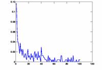
We plotted some histograms and graphs indicating the height and position of the peak using delayplots.m. Delay histograms showed a wide variety of distributions. The most prominent peak was more than 65%, there also were relatively many between 10% and 20%. Some histograms did not show any significant peak. The arising question is when to infer an edge between the two nodes. We decided to use a fixed threshold to make this decision. Naturally, this threshold greatly influences the outcome of the connectivity graph. If the threshold is too low, every node pair meets the condition, the result is a fully connected graph. On the other hand, if the threshold is too high, no channel pair meets the requirement and the graph has no edges at all. To be flexible, we used the script show_graph_d.m to plot the results of the edge inference algorithm for various thresholds. The network characteristics L and C are also computed in this script and printed on the graph. The degree distribution P(k) is plotted in a separate graph.
To establish a comparison between the inferred network and random networks, we computed two different random networks for each inferred network.
First, we create a random network in the classic sense by computing a graph that consists of the same number of nodes as the inferred one and the same number of edges. The position of the edges, however, is completely random. In show_graph_d2.m and show_graph_draw.m, the inferred network along with its random version is plotted.
Additionally, to test for possible artifacts of our edge inference method, we create random spike trains with the same average spiking probability as the MEA data and run our inference algorithm on this artificial data using rndspikes.m, delaycomp_r.m and show_graph_dr.m.
Cross-Covariance
(xcov) method of edge determination
A second method to determine edges is to use the covariance between channels. Intuitively, we could expect some a connection from channel A to channel B if there is always a flurry of activity on channel B at some particular time (within a certain window) after every spike on channel A. If there is some consistent and repeatable pattern to this activity, it will show up as a peak in the covariance graph. However, if the spiking patterns are completely random, the covariance graph should be flat.
In contrast with the previous method, this relaxes the condition that a consistent timing pattern must be observed on only the first spike on channel B after a spike in channel A occurs. This could be a more realistic measure to use, because an electrode may be sitting over several neurons, and these neurons may be receiving other spikes or even be spiking spontaneously. Thus it is conceivable that if a neuron under channel A is connected to a neuron under channel B, channel B may be spiking for many other reasons in the intervening time before its response to channel A is picked up. And as the electrodes are spaced 100um apart, it is conceivable that the connection time to reach channel B is not bounded by a single synaptic transmission but over several transmissions. The longer the transmission time, the more likely there will be additional spiking during the intermission. Thus if we only look at the first spike timing on channel B, we could miss several notable responses to channel A. The extent to which these conditions may be true could be highlighted by a comparison between the two methods. However, the first order of business was to see if our network characterization would be robust to two different methods of edge-determination.
To compute the covariance matrix, we first needed to fill 64 vectors (1 for each channel) with digital impulses accumulated at each spike time. One important question is how finely the time-steps should be spaced. A 1ms time-step was tried, and compared to a 10ms time-step. We suspected that a 10ms time-step would work better because it would not require the spikes to arrive exactly within the same millisecond in order for there to be a positive covariance. And indeed, allowing for some play in arrival time produced more significant peaks and valleys in the covariance graphs.
However, while there is rarely more than 1 spike in a 1ms time bin (and at most 2, since we use 0.4ms windowing to look for spikes in the voltage waveform), there could be several spikes in a 10ms time bin. Hence we needed to accumulate all the spikes within 10ms into a single point. This causes a problem that spikes arriving at the edges of a 10ms window may still miss each other and not be correlated if they straddle different bins. Hence we made an extra 2ms on each edge of a 10ms bin to overlap with one another, and weighted this overlap so that their effect would be spread equally between the 2 bins. The code to do this binning and to compute the cross-covariance matrix is in the script spikes3.m.
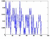
Once the cross-covariance matrix was obtained, covariance plots of each channel pair were made by the script plot_xc.m. For N channels, there are N(N-1)/2 possible combinations (or 2016 for 64 channels, and 231 for just 22 channels) so we could only check a fraction of the total number of plots to get an idea of what the graphs looked like. A sample set of some channel pairs from 49 to 64 is shown below:
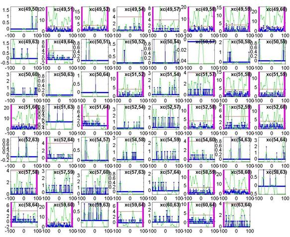
The blue plot is the cross-covariance of the 1ms-binned spike train, while the green plot is the cross-covariance of the 10ms-binned spike train. A lag window of 100ms (from -100ms to 100ms on the x-axis) is used. As predicted, the peaks are much more significant when using the green 10ms bins. By eyeballing several plots like these, an arbitrary threshold of about 4 was used to determine edges. If the green plot exceeded the threshold (shown as a horizontal red line), we declared a connection to exist. For xc(A,B) if the green plot exceeds the threshold at a positive time lag, then a directed edge from A ® B is created, and shown as a magenta bar on the right. If the green plot exceeds the threshold at a negative time lag, then a directed edge from B ® A is created, and shown as a magenta bar on the left.
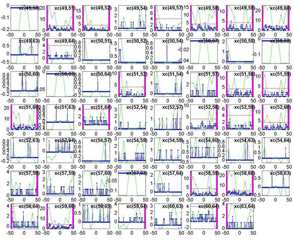
Shown below is the output of plot_xc.m using a lag window of 50ms instead of 100ms. As expected, fewer edges are declared because we look over a shorter time to find a significant peak.
A final note on this method: we found it is important to use the cross-covariance rather than the cross-correlation, because the covariance subtracts the mean from the binary signal to weight the quiet regions negatively. If the quiet regions are not negatively weighted, any spiking regions which line up on occasion but show no consistent behavior will not be penalized. This means a very active channel spiking completely at random will end up showing a higher degree of correlation than a very quiet channel even though they may be spiking equally randomly.
Results
Results from delay histogram method
We generated plots for threhsolds in the range of 1% to 40%. As outlined before, at the ends of this spectrum, the inferred graphs were trivial. In the middle range between 10% and 20%, inferred graphs were obviously different from both empty and fully connected graphs.
These are the inferred network and its random network comparison graph for a threshold of 10%. While L is in the same range for both graphs, C is significantly smaller for the random graph on the right.
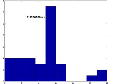
The degree distributions for the above shown networks show very different behavior. While the random network’s distribution is similar to a Poisson distribution, the inferred network’s degree distribution resembles neither a Poisson nor a power law distribution.
These graphs show the inferred network for a threshold of 15% (upper left) along with its random network (upper right) and the corresonding degree distributions. Again, L are in the same range, C is much higher for the inferred network and the degree distributions follow the same pattern as for a threshod of 10%.
Random spike trains
As discussed in the methods, we also created random spike trains and ran our algorithm on these random data. As expected, the thresholds had to be set much lower in order to yield networks that are neither fully connected nor almost empty. The graphs below show the result for a threshold of 4%. Note that the average path length is in the same range as for all the previous graphs while the average connectivity is much lower than for the networks inferred from the MEA data. Interestingly, the degree distribution bears a striking resemblance to a power law distribution with g » -1.
Results from cross-covariance method
The network characteristics of L, C and P(k) are calculated from the cross-covariance matrix by the following scripts: show_graph.m, ShortestPath.m.
The function definition for show_graph.m is:
function
show_graph( nodelist, xc_len, threshold, num_std, fig )
The parameters xc_len, threshold and num_std allow us to use various lag windows, thresholds for determining an edge, and the number of standard deviations used in thresholding for a spike.
Graphs using various parameters were generated to see how sensitive our data was to the choice of these parameters, since (as noted before) they are chosen rather arbitrarily, by eyeballing the curves for reasonable levels.
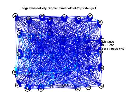
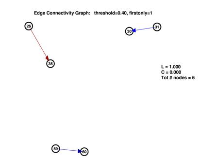
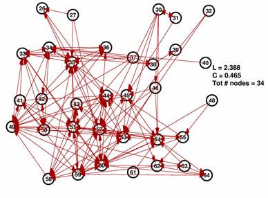
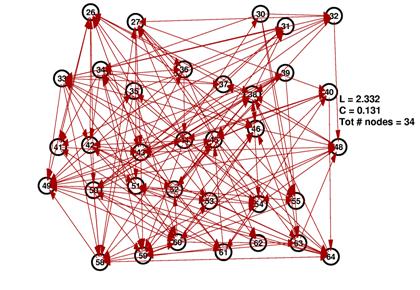
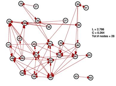
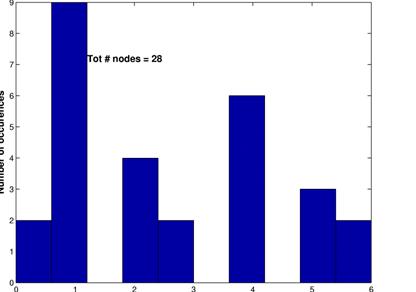
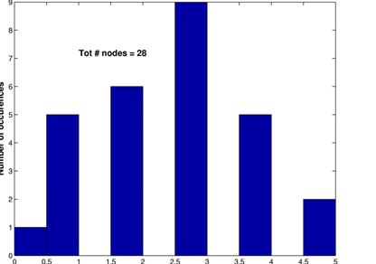
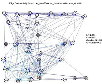
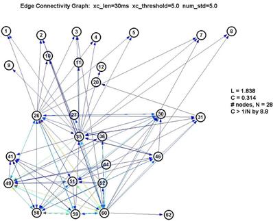
Fortunately, it turns out that the characteristic L and C are largely unaffected by our choice of parameters. This is significant because it gives us a good deal of confidence that the results are robust. If we use a shorter lag window (to look over less than 100ms) or a higher threshold (to create fewer edges) we will create a graph with fewer connected nodes (some nodes simply drop out of the graph) ― but of the remaining nodes, L and C remain roughly unchanged. This is shown in the 3 plots below:
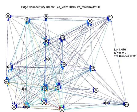
The color of the edges reflects the size of the peak in the xcov() curve above the threshold, with red being largest and blue being smallest.
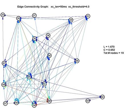
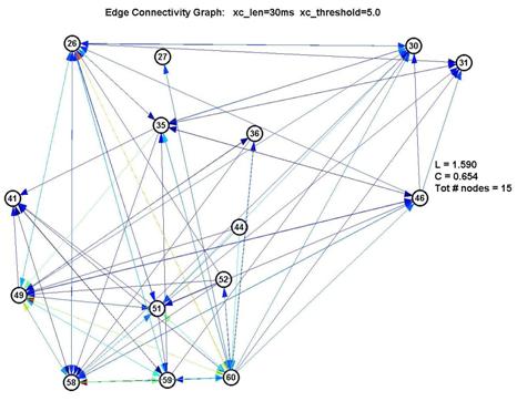
Thus L remains pegged around 1.5-1.7, which is low for a graph of 15-22 nodes, and C remains around 0.6-0.7, which is over 10× higher than 1/N (where N is the number of nodes). This is a significant measure because a purely random network is characterized with a value of C on the order of 1/N.
As for the degree distribution, our results are unfortunately inconclusive, because of two reasons mentioned earlier: (1) we have a very small number of nodes to work with, and (2) the assumptions of node growth / preferential attachment to nodes of high degree may not be valid.
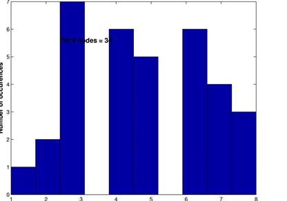
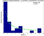
However, we present the histograms corresponding to the 3 plots above, to show the various profiles of P(k).
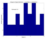
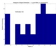
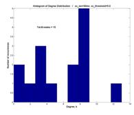
And the shape of P(k) may vaguely suggest a Poisson distribution characteristic of networks that employ random attachment ― a peak centered at (in this case, near) the mean, and a rolloff (although not exponential) away from the peak ― rather than an inverse power law P(k) µ k-g.
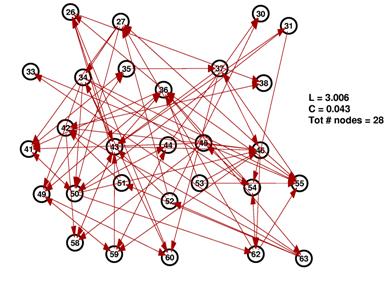
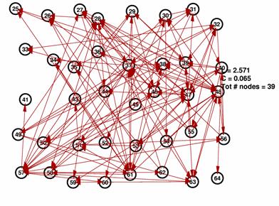
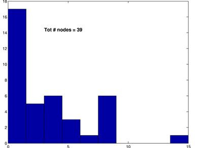
However, if we include all 64 nodes in the graph, then P(k) indeed starts to look more like an inverse power law with g » -1.
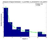
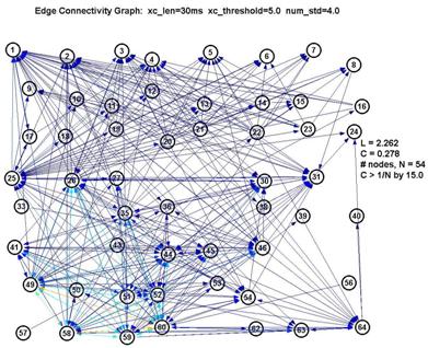
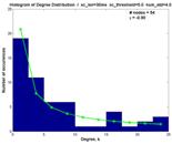
However as seen by the graph above with xc_len=30ms, xc_threshold=5.0 and num_std=5.0, the large number of nodes with low degree are contributed by the nodes 1-24. They also inflate the degree of the nodes from 25-64 (especially 26, 35 and 60). Thus whether the degree distribution truly follows a power-law here is suspect.
Discussion
Intuitively, we can think of L to measure the sparsity of long-range connections and C to measure the degree of interconnectedness within the network. Small-world networks are characterized by small L because their density of long-range connections is sufficient to lower L while the network still remains far from being fully-connected. Small-world networks also have C at least an order of magnitude larger than 1/N, where N is the number of nodes, distinguishing it from a random network.
Our results have shown that L is consistently low, between approximately 1.5 - 3, regardless of:
(1) the method of edge determination (2 methods were considered)
(2) the parameters used to determine edges (such as window size and threshold), or
(3) the spike extraction threshold
― all of which caused the number of nodes in the graph to vary greatly, from as low as 15 to over 50. Having a L of 1.5 for a 15 node graph may not seem impressive at first, but having that remain at around 2 for a 54 node graph is certainly significant.
Results also show C to be large, and as robust to method and parameter variation as L, when we look at the number of times C is larger than 1/N (by taking the C×N product). The C×N product is consistently large and varies over a small range (from 9 to 17). Together with the one-to-one comparison random networks, this shows that the underlying network is clearly non-random in this regard.
It would be premature to confirm or deny a scale-free nature in this network, based on our measurements of the degree distribution. The degree distribution suffers primarily from being limited in size, as the degrees considered in real world networks span 3 or 4 orders of magnitude, while our network hardly spans more than 1. We would expect that the network is NOT scale-free, however, because the assumption of the addition of nodes after a par of the network is already established does not hold for our case. Additionally, we do not expect neurons to know about the connectivity of other neurons when they are growing all their connections brand new. This might actually be the case using chemical gradients etc., but more research has to be done on this issue. If there was more data available and we would observe a power-law distribution, this could actually spark new experiments on this question, supporting the existence of some ‘guiding’ substance for axon growth.
Future work to tease apart the electrode-to-neuron mapping would likely shed more light on the entire MEA dataset. Perhaps this could be done at the experimental level with finer spaced electrodes or limiting the growth of intentional neurons beneath each electrode. The principal component analysis and spike sorting algorithms presented by other groups also move in this direction from an analysis standpoint.
References
- Panasonic (2003). MED64 Systems
- Multichannel Multielectrode Array Systems for In-vitro
Electro-physiology. Retrieved
- D.J. Watts, S.H. Strogatz (1998): Collective dynamics of 'small-world' networks. Nature 393.
- A.-L. Barabasi, R. Albert (1999): Emergence of scaling in random networks. Science. 286.
- X.F. Wang, G. Chen (2003):Complex networks: small world, scale free and beyond. IEEE Circuits and Systems Magazine I/2003.
- M.E.J. Newman (2002):Random
graphs as models of networks. Santa Fe Institute Working Paper
- L.A.N. Amaral, A. Scala, M.Barthelemy, H.E. Stanley (2000): Classes of small world networks. PNAS 97(21).
Contributions
Both authors contributed to every stage of the project. For the final implementations, Ji-Jon Sit focused on the initial data cleaning and filtering as well as the cross-covariance approach to connectivity inference and the computation of the network parameters. Ulf Knoblich led the literature review and implemented the delay histogram approach and the random networks for comparison. These contributions also extend to the passages of this article about the respective topic.