| Home | Publications | Personnel | Models | Outreach | Structure | SEARCH |
|
|
| Home | Publications | Personnel | Models | Outreach | Structure | SEARCH | |
The MIT Integrated Global System Model: Climate Component
To represent the dynamics of climate within the MIT Framework, an initial task was to develop a computationally efficient model capable not only of simulating reasonably well the present climate but also of reproducing the climate change patterns predicted with 3D GCMs. The current MIT climate model couples a two-dimensional (2D) land- and ocean-resolving (LO) statistical-dynamical model of the atmosphere to a 3D ocean general circulation model (GCM). An atmospheric chemistry model and the 2D-LO climate model are coupled to run interactively and simultaneously, to provide predictions of the atmospheric concentration of radiatively and chemically important trace species. Details of the individual model components are provided in several publications.
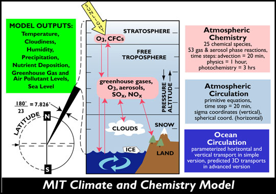
The MIT climate model, with its 2D atmosphere/3D ocean, is capable of reproducing many characteristics of the current longitudinally-averaged climate, and its behavior and predictions are similar to those of more complex, fully 3D GCMs. Most significantly, it is twenty times faster than 3D models with similar latitudinal and vertical resolutions. Utilizing the simplified (2D atmosphere/3D ocean) climate model structure has allowed the Program to perform multiple model runs which provides a facile investigation of feedbacks between model components. The simplified climate component enables extensive testing of these phenomena, which would not be practical in a calculation incorporating a 3D chemistry/climate model. A 100-year integration of the latest version of the climate model requires 10 hours on a single 500 MHz CPU.
The MIT atmospheric model is a modified version of an atmospheric GCM developed by scientists at MIT and the NASA Goddard Institute for Space Studies (GISS). It is a 2D (zonally averaged) statistical-dynamical model that solves the zonally averaged primitive equations in latitude-pressure coordinates. The model's grid is variable, but in the standard version contains 46 points in latitude, corresponding to a resolution of 4.0 degrees, and 11 layers in the vertical. The model's numerics and most of the parameterizations of physical processes closely parallel those of the GISS GCM. The radiation code used in the model includes all significant greenhouse gases (H2O, CO2, CH4, N2O, CFCs, O3, etc.) and different types of aerosols. The MIT 2D atmospheric model also includes parameterizations of heat, moisture, and momentum transports by large-scale eddies. The model has complete moisture and momentum cycles and reproduces most of the non-linear interactions and feedbacks simulated by atmospheric GCMs. The atmospheric model's climate sensitivity can be changed by varying the cloud feedback.
The MIT 2D model allows four different types of surfaces in the same grid cell, namely open ocean, sea-ice, land, and land-ice. The surface characteristics as well as turbulent and radiative fluxes are calculated separately for each kind of surface, while the atmosphere above is assumed to be well-mixed zonally. More detailed descriptions of the atmospheric model component can be found in Sokolov & Stone (1998) and Prinn et al. (1999).
The 2D atmospheric model, coupled to a simple Q-flux mixed layer/diffusive ocean model, has been shown to reproduce, with an appropriate choice of the model's cloud feedback and effective diffusion coefficient, transient surface warming and sea level rise due to thermal expansion of the ocean as simulated by different coupled atmosphere-ocean (AO) GCMs for 120-150 years. Such a model cannot however represent feedbacks associated with changes in the ocean circulation. To take into account possible interactions between atmosphere and ocean circulation, the diffusive ocean model is replaced in some studies by a 3D ocean GCM with simplified geometry (described next).
The 3D ocean component of the coupled climate model in the MIT IGSM2 uses the z-coordinate MIT ocean GCM developed by the MIT Climate Modeling Initiative. A uniform horizontal resolution of 4 degrees in both latitude and longitude is used (90 x 44 grid points), which allows for a realistic, albeit crude, depiction of the Earth's bathymetry, including a representation of the Arctic Ocean. The model has 15 layers in the vertical with thicknesses increasing downward from 50 to 500 meters. The model is run using asynchronous integration, with a momentum time step of 15 minutes and a tracer timestep of 12 hours.
The ocean model is hydrostatic and Boussinesq. No-slip conditions for horizontal velocity are applied at the lateral walls with free-slip conditions are used at the bottom. Boundary conditions for tracers are insulating at lateral walls and bottom. We employ the Gent-McWilliams scheme for the parameterization of eddy transports of tracers. Mixing coefficients in the reference version are 1 x 10⁴ and 0.01 m2/sec for horizontal and vertical viscosity, and 3 x 10⁻⁴ m2/sec for vertical tracer diffusivity. Isopycnal diffusivity and isopycnal thickness diffusivity coefficients are both 103 m2/sec, with tapering occurring using the Gerdes et al. (1991; Climate Dynamics, vol. 5) method with maximum slope 0.01. A simple diffusive convective adjustment procedure occurs if and when static instability is present. Multiple versions of the ocean model are created using various choices for the uncertain parameters.
Ocean Carbon Component
![]()
The ocean carbon model solves continuity equations addressing the movement of total dissolved inorganic carbon (DIC) within the ocean and the exchange of carbon with the atmosphere. The physical ocean model velocity and diffusivities are used to redistribute DIC within the ocean. Air-sea exchange of CO2 is parameterized following Wanninkhof (1992). Surface ocean pCO2 is determined from local DIC, alkalinity, temperature, salinity, borate, phosphate and silica concentrations following the algorithms used in the ocean carbon modeling intercomparison project (OCMIP). Borate and silica are assumed constants, but the remaining variables are carried as tracers in the model. We include the effect of the biological pump; biological production in the surface waters is calculated as a function of light and nutrient (phosphate) availability (similar to McKinley et al., 2004). A portion of this biological matter sinks from the surface and remineralizes at depth. The impact of carbonate chemistry is also taken into account following Najjar & Orr (1998).
Sea-Ice and Glacial-Ice Components
![]()
Both the atmospheric and ocean models are coupled to a thermodynamic ice model used for representing sea ice. In addition, the climate model includes a physically-based snowpack model of the mass balance of the Greenland and Antarctic ice sheets. The sea-ice model solves equations for conservation of enthalpy, and is based on CICE, and Winton (2000). The model has three layers (two ice layers and a snow layer) and computes ice concentration (the percentage of area covered by ice for a given grid cell) and ice thickness. A realistic treatment of sea-ice brine content is included in the model.
Atmospheric Chemistry Component
![]()
To calculate atmospheric composition, the model of atmospheric chemistry includes analysis of the climate-relevant reactive gases and aerosols at urban scales, coupled to a model of the processing of exported pollutants from urban areas (plus the emissions from non-urban areas) at the regional to global scale. For calculation of the atmospheric composition in non-urban areas, the climate model is linked to a detailed 2D zonal mean model of atmospheric chemistry. The model's grid is variable, but in standard version it contains 46 points in latitude, corresponding to a resolution of 4°, and 11 layers in the vertical.
Urban airshed conditions are resolved at low, medium and high levels of pollution. The reduced-form urban air chemistry model provides detailed information about particulates and their precursors. The structure takes account of pollutant properties important to human health, and of the effects of local topography and possible urban development scenarios on the level of containment and thus intensity of air pollution events. This is an important consideration since air pollutant levels are highly dependent on projected emissions per unit area, not just total urban emissions.
The 2D zonal mean model that is used to calculate atmospheric composition is a finite difference model in latitude-pressure coordinates, and the continuity equations for trace constituents are solved in mass conservative or flux form (Wang et al., 1998). The local trace species tendency is thus a function of convergence due to 2D advection, parameterized north-south eddy transport, convective transports, local true production or loss due to surface emission or deposition, and atmospheric chemical reactions. The model includes 33 chemical species (among them CO2, CH4, N2O, O3, CO, H2O, NOx, HOx, SO2, sulfate aerosol, CFCs, HFCs, PFCs, SF6, black carbon as well as organic carbon aerosols).
The chemical reactions are processed in two separate modules: one for the 2D model grids and one for sub-grid urban fast chemistry. There are 41 gas-phase and 12 heterogeneous reactions in the background chemistry module applied to the 2D model grid. The sub-grid fast urban chemistry module is a reduced format model derived by fitting multiple runs of the detailed 3D California Institute of Technology (CIT) Urban Airshed Model (Mayer et al., 2000). The continuity equations for CFCl3, CF2Cl2, N2O, O3, CO, CO2, NO, NO2, N2O5, HNO3, CH4, CH2O, SO2, H2SO4, HFC, PFC, SF6, black carbon aerosol, and organic carbon aerosol include convergences due to transport whereas the remaining very reactive atoms, free radicals, or molecules are assumed to be unaffected by transport because of their very short lifetimes. Scavenging of carbonaceous and sulfate aerosol species by precipitation are also included using method derived based on a 3D climate-aerosol-chemistry model (Wang, 2004). Water vapor and air (N2 and O2) mass densities are computed using full continuity equations as a part of the climate model to which the chemical model is coupled. The climate model also provides wind speeds, temperature, solar radiation flux and precipitation which are used in the chemistry formulation.
Atmospheric-Ocean Coupling Procedure
![]()
Coupling of the atmosphere and ocean model components takes place once a day. The atmospheric model calculates 24-hour means of heat and fresh-water fluxes over the open ocean, and a heat flux over sea ice, as well as their derivatives with respect to surface temperature and the wind stress. The partial derivative of upward longwave radiation is calculates as 4σT3, where σ is the Stephan-Boltzman constant. Fluxes of sensible and latent heat are calculated in the atmospheric model by bulk formulas with turbulent exchange coefficients dependent on Richardson number. The atmosphere's tubulence parameterization is also used in the calculation of the flux derivatives. Total heat and fresh-water fluxes for the ocean model vary by longitude as a function of ocean sea surface temperature, i.e., warmer ocean locations undergo greater evaporation and receive less downward heat flux. The wind stress values applied to the ocean are zonally uniform. A more detailed discussion of technical issues involved in the calculations of these fluxes and their derivatives is given in Kamenkovich et al. (2002). After receiving these fluxes from the atmosphere, the ocean and sea-ice models are integrated for 24 hours (two ocean tracer time steps). At the end of this period, sea surface and surface ice temperatures are passed back to the atmospheric model.
|
|
|
Comments and questions to
globalchange@mit.edu
1/2006 Copyright © 2006 Massachusetts Institute of Technology | |