Snowpack model

A complete approach to modeling the temperature and density distribution of a snow, firn and ice mixture would require a three phase, four-component system: Liquid water, water vapor, ice and air (Morland et al. (1990)). Simplified models with two or three components have been developed for avalanche forecasting purposes in the Alps (Brun et al. (1989), Bader and Weilenmann (1992)) or to describe the evolution of the seasonal snowcover (Anderson (1976); Loth and Graf (1993)). A similar modeling approach is used here to estimate the mass balance of the Greenland and Antarctic ice sheets. Because snowpack models are based on physical principles, it is believed that their response to changes in the climatic forcing is appropriate. This is not the case for parameterizations which are calibrated to a certain range of climatic conditions.

The model described in the following paragraphs is one-dimensional in the vertical direction, it treats the uppermost 15 meters of the snow/firn/ice as a two component system: Liquid water and snow. Ice and air are treated jointly as snow of variable density. Although the firn air is saturated with water vapor, the contribution of sublimation/fusion to the energy and mass balances can be shown to be negligible (Bader and Weilenmann (1992)). Liquid water can only be present if the snow is at the melting point and is absent at lower temperatures. This common temperature of the water/snow mixture presents the advantage of reducing the problem to a single thermodynamic equation for both components.

The momentum balance for snow can be reduced to a hydrostatic balance with the atmospheric pressure serving as surface boundary condition. The constitutive relation for snow - relation between the deformation or strain rate and the imposed stress - is derived from observations of the rate at which snow settles under the pressure of the overlying layers. Snow is best described as a compressible viscoelastic material in which the viscosity is both density and temperature dependent (Male (1980)). This yields the following rate of change in the thickness, h, of a layer of snow:

 

$${\frac{d}{d \,z}} \left(\vphantom{ \frac{d \,h}{d \,t} }\right. {\frac{d \,h}{d \,t}} \left.\vphantom{ \frac{d \,h}{d \,t} }\right) {\frac{\sigma_{s}}{\eta}}$$ (2)

$$\eta \rho_{s}^{} \rho_{s} {\frac{6042}{T}}$$ (3)

where the temperature T is in Kelvin and $\sigma_{s}^{}$ is the snow load. The compaction viscosity, $\eta$, which is used in this model was derived empirically from measurements in Greenland and Antarctica (Male (1980), Morris et al. (1997)). Although small, the vertical velocity due to snow settling, w_s, can easily be retrieved from the change in layer depth.

Two mass conservation equations for the density of snow, $\rho_{s}^{}$, and its water content, $\theta$, are required to translate the phase changes between the components into density changes.

$${\frac{d \rho_s}{d\,t}} {\frac{\partial \rho_s}{\partial t}} {\frac{\partial \rho_s}{\partial z}}$$ (4)

$${\frac{d \theta}{d\,t}}$$ (5)

m_{s - w} is the melting rate per unit volume.

The mass balance for liquid water must take into account the percolation of water between the layers. Drainage is modeled by a simple maximum retention capacity model: The water in excess of a prescribed volume fraction percolates to the lower layer. The reference value chosen for this so-called ``irreducible water saturation'' is 3% per unit volume (Male (1980)). A more complicated Darcy type flow law as the one proposed by Colbeck (1972) would be more accurate but its implementation requires a timestep too short for our modeling objectives. Horizontal movement of the meltwater is neglected on the grounds that any liquid water flowing down the slope of the ice sheet will generally encounter areas in which the firn is already saturated with water and will not refreeze. Once formed, the runoff is therefore assumed to reach the ocean.

The snowpack model is initialized by prescribing a uniform temperature distribution and a density profile increasing linearly from the surface to 15m depth. The time taken for the snow cover to equilibrate with the current climate and develop realistic density and temperature profiles varies with the location on the ice sheet and can take up to a century.

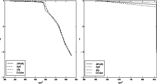
Fig.1 represents the seasonal evolution of two density profiles, one at the Carrefour site in the accumulation zone (left-hand figure), the other at Nordbogletscher in the ablation area of the Greenland ice sheet. These profiles were obtained by using the surface forcing of the MIT climate model's representation of the current climate (see Section 3 for a description of the climate models). The density increase in the accumulation zone is gradual and the transition to ice occurs below 15 m., at depths between 40 and 115 m depending on the accumulation rate and the surface temperature (Paterson (1994)). Fresh snow is added at a density of 320 kg m^-3, a value which is usually reached in polar snow after less than a day of settling (Morris et al. (1997)). In the ablation region (right-hand figure), the ice is covered with a thin cover of snow which gradually thickens during the fall, winter and spring seasons. As shown by the July curve (dash-dotted line), bare ice is exposed at the surface during the summer.

  

Figure: Model depth Profiles (in m) of the snow/ice density (in kg m^-3) for January, April, July and October. Left: Carrefour ( 69^o50'N;45^o25'W;1850 m, Greenland). Right: Nordbogletscher ( 61^o28'N;45^o20'W;880 m, Greenland). The figures are plotted on different scales for clarity. The climate forcing is derived from the MIT model simulation of the 1990 climate.

The temperature, T, within the snow pack is determined by heat diffusion and by the changes of phase of water.

$${\frac{\partial T}{\partial t}} {\frac{\partial }{\partial z}} \lambda_{\mathit{eff}}^{} {\frac{\partial \,T}{\partial z }}$$ (6)

The effective heat capacity, Cp_eff, and thermal conductivity, $\lambda_{\mathit{eff}}^{}$, take into account the mass fraction of snow and water in the mixture. L_{s - w} is the latent heat of fusion and m_{s - w} represents the mass of water per unit volume which changes phase at a given timestep. A scale analysis of the generalized thermodynamic equation shows that the advection of heat by snow settling or water percolation is smaller than the other terms. The penetration of shortwave radiation in the snowpack is attenuated completely within the uppermost centimeters of the snow, and has therefore been neglected, as has the effect of wind pumping on the sensible heat loss within the snowpack.

This diffusion equation being of second order in space, two boundary conditions are required to obtain a solution. Since the annual temperature cycle is damped within the uppermost meters of the snowpack, a vanishing heat flux at 15 m depth provides an excellent lower boundary condition, even when integrating the model forward over a century. The surface energy balance - sum of the net shortwave Q_SW and longwave Q_LW radiative fluxes and of the turbulent latent Q_LAT and sensible Q_SENS heat fluxes - can be used to calculate the heat flux through the surface of the ice sheet:

$$\left.\vphantom{ \lambda_{eff} \frac{\partial T}{\partial z} }\right. \lambda_{eff}^{} {\frac{\partial T}{\partial z}} \left.\vphantom{ \lambda_{eff} \frac{\partial T}{\partial z} }\right\vert _{z=0}^{}$$ (7)

The downwelling shortwave radiation must be available from measurements or from an atmospheric model output. The net absorbed shortwave radiation can be determined if the surface albedo, $\alpha$, is known or prescribed. The albedo parameterization used in this model includes a dependence on the time elapsed, t here in days, since the previous snowfall (Loth and Graf (1993)),

$$\alpha \alpha_{0}^{}$$ no melting

$$\alpha \alpha_{0}^{}$$ melting period (8)

and takes advantage of the strong correlation between the albedo of snow and ice and the air temperature (Kang (1994)). Ice is assumed to have a constant albedo (Knap and Oerlemans (1996)):

$$\alpha_{0}^{}$$ -10 < T_air < 0^oC cold snow

$$\alpha_{0}^{}$$ 0 < T_air < 8^oC temperate snow

$$\alpha_{0}^{}$$ ice (9)

The upwelling longwave radiation can be calculated by assuming that the snow cover emits as a blackbody, the downwelling component must be provided as input.

The latent and sensible heat fluxes are parameterized with the bulk transfer formulae described in Hansen et al. (1983) and Sokolov and Stone (1995). Different roughness lengths for cold, temperate snow and ice, z_cold snow = 0.12 ^. 10^-3 m, z_{temperate snow} = 1.3 ^. 10^-3 m and z_ice = 3.2 ^. 10^-3 m are used in the calculation of the bulk transfer coefficients (Greuell (1992)). The assumption of a constant 70% relative humidity is used to derive the air specific humidity required for the calculation of the latent heat flux. Although this value is lower than most reports by stations located near the coast, it is not inconsistent with values measured inland (Schwerdtfeger (1970)). It furthermore gives latent heat fluxes which are in agreement with observations.

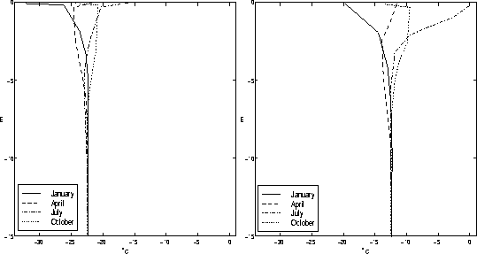
The seasonal variation of two temperature profiles on the Greenland ice sheet, as predicted by the snowpack model for the current climate, are shown in Fig.2. There is a strong coupling between the surface snow temperature and the air temperature at the Carrefour site in the accumulation zone (left-hand figure), and the annual temperature cycle is rapidly damped with depth. The convergence of the seasonal temperature profiles by a depth of 10 m validates the use of a vanishing heat flux at 15 m as lower boundary condition. The profiles on the right-hand side of Fig.2 are representative of the ablation zone (Norbodgletscher). The uppermost centimeters of the snow/water mixture in the July profile (dash-dotted line) are temperate while the lower part remains below the freezing point. The temperature inversion which develops in October is a common characteristic of both temperature profiles.

  

Figure 2: Model depth Profiles (in m) of the snow/ice temperature (in ^oC) for January, April, July and October. Left: Carrefour ( 69^o50'N;45^o25'W;1850 m, Greenland). Right: Nordbogletscher ( 61^o28'N;45^o20'W;880 m, Greenland). The climate forcing is derived from the MIT model simulation of the 1990 climate.

The numerical procedure used to calculate the temperature distribution is the Crank-Nicholson scheme which is unconditionally stable for a dry snowpack, yet requires the convergence procedure described by Bader and Weilenmann (1992) to ensure an accurate calculation of the mass of water which is melted or frozen at each timestep. The timestep is determined individually at each grid point by the total amount of melting experienced during the previous year. This guarantees an optimal accuracy for the points in the ablation zone which require a shorter timestep because of melting and percolation and an efficient scheme in the accumulation zone. The timestep therefore varies between 1 hour and 1 day depending on the location on the ice sheet.

Snow or ice of a density and temperature equivalent to that of the lowest model layer is added or subtracted to the column at each timestep in order to maintain a constant total thickness of 15 m. Because of the snow settling process, the layers do not maintain a constant thickness and are combined or divided at every timestep to ensure smooth density and temperature profiles.