
October 1998
Marginal abatement curves (MACs) are often used heuristically to demonstrate the advantages of emissions trading. In this paper, the authors derive MACs from EPPA, the MIT Joint Program's computable general equilibrium model of global economic activity, energy use and CO2 emissions, to analyze the benefits of emissions trading in achieving the emission reduction targets implied by the Kyoto Protocol. The magnitude and distribution of the gains from emissions trading are examined for both an Annex B market and for full global trading, as well as the effects of import limitations, non-competitive behavior, and less than fully efficient supply. In general, trading benefits all parties at least some, and from a global standpoint, the gains from trading are greater, the wider and less constrained is the market. The distribution of the gains from trading is, however, highly skewed in favor of those who would face the highest costs in the absence of emissions trading.
1. BACKGROUND, PURPOSE OF THE STUDY
At the Third Conference of the Parties (COP-3) to the United Nations Framework Convention on Climate Change (UNFCCC), held in Kyoto in December, 1997, Annex B parties[1] agreed to CO2 emissions ceilings for the years centered on 2010, but left many details to be decided through further negotiations and subsequent COPs. In particular, the extent to which parties could resort to emissions trading to meet their commitments is to be addressed at COP-4 in Buenos Aires in November, 1998.
This paper provides an analysis of the importance of emissions trading by using marginal abatement curves (MACs) generated by MIT's Emissions Prediction and Policy Analysis (EPPA) model. These cost curves can be used to determine marginal, average and total cost, but more importantly they can indicate the potential gains from emissions trading for various parties and the extent to which those parties would wish to resort to emissions trading. The effect of constraints on the selling or buying of tradable carbon permits can also be illustrated. Thus, this paper attempts to clarify what is at stake at in Buenos Aires and in subsequent negotiations to determine the role of emissions trading in a global carbon regime.
EPPA is a multi-regional, multi-sectoral Computable General Equilibrium (CGE) model of economic activity, energy use and carbon emissions.[2] The acronyms for the twelve regions are indicated below. The six regions listed on the left are Annex B regions; the other six are non-Annex B regions. The study takes the year 2010 as representative of the first commitment period, which includes the years 2008 through 2012. The model keeps track of five vintages of capital. Version 2.6 of the model, which is used here, incorporates two backstop technologies; however, because these energy sources will not play a substantial role in 2010, they are omitted from the calculations presented here.
Definitions of Regions in the EPPA Model
ANNEX B REGIONS:
NON-ANNEX B REGIONS: USA: USA
EEX: Energy Exporting Countries
JPN: Japan
CHN: China
EEC: European Union (EC-12 as of 1992)
IND: India
OOE: Other OECD Countries
DAE: Dynamic Asian Economies
EET: Eastern Europe
BRA: Brazil
FSU: Former Soviet Union
ROW:Rest Of World
The carbon emission reduction constraints used for this study are based on the commitments made by the various Annex B parties to the Kyoto Protocol. Table 1 states these commitments for the regional aggregates used in EPPA, indicates the reference (or business-as-usual) emissions for the year 2010 as predicted by EPPA version 2.6, and calculates the absolute and percentage reductions required to meet the Kyoto Protocol commitments.[3]
Table 1. Emissions Levels Corresponding to Kyoto Commitments
USA
JPN
EEC
OOE
EET
FSU
Non-Annex B
Reference emissions 1990 (Mton)
1362
298
822
318
266
891
2022
Reference emissions 2010 (Mton)
1838
424
1064
472
395
763
4142
Kyoto commitments / 1990
93%
94%
92%
94.5%
104%
98%
NA
Hence Emissions Target in 2010 (Mton)
1267
280
756
301
273
873
4142
i.e. Reduction / ref (Mton)
571
144
308
171
118
0
NA
i.e. Reduction / ref (%)
31%
34%
29%
36%
30%
0
NA
`hot air' (Mton)
0
0
0
0
0
111
NA
The next section of this paper concerns methodology; it explains marginal abatement curves and how they are generated by Computable General Equilibrium (CGE) models, such as EPPA. In particular, we explore the robustness of these MACs, that is, whether the abatement costs for a given region are invariant with respect to abatement in other regions.
Section 3 presents three illustrative cases in which the scope of the market is progressively widened from no trading to full global trading. Perfectly competitive markets are assumed both to simplify the presentation and to illustrate the maximum gains from emissions trading. We also discuss `hot air' and `leakage' in this section.
In Section 4, we examine several departures from the simplifying assumptions of perfect competition to impart a more realistic light on the potential gains from emissions trading. In particular, three departures are examined: import limits, non-competitive behavior, and inefficiencies in supply. The final section gathers the main findings of the study, in terms of both methodology and policy analysis, and suggests future extensions of this research.
2. METHODOLOGY: Using the MACs Generated by the EPPA Model for Trade Studies
2.1 What are Marginal Abatement Curves and What Do They Represent?
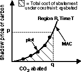
A CGE model will produce a shadow price for any constraint on carbon emissions for a given region R at time T. An example would be a 10% reduction below the reference case for the USA in 2010. This price indicates the marginal cost for reducing or abating the last ton of carbon required to meet the constraint. As might be expected in a proper CGE model, the shadow prices corresponding to constraints of increasing severity rise as an increasing function of emissions reduction.
A Marginal Abatement Curve plots the shadow prices corresponding to constraints of increasing severity at time T against the quantity abated. One point (q, p) on the curve thus represents the marginal cost for region R of abating an additional unit of carbon emissions at quantity q in time T. Figure 1 shows such a Marginal Abatement Curve. The integral under the curve (hatched area) represents the total abatement cost for region R of carbon emission reduction q at time T.

Figure 1. Marginal Abatement Curves.
2.2 How Can MACs Be Used for Trade Studies?
Any emission reduction for a region can be represented as a point on its marginal abatement curve. If several regions commit to achieve emission reductions at the same time, and if the marginal costs associated with those reductions are different, the aggregate cost of meeting the commitments will be less to the extent that a region with higher marginal costs can induce a region with lower marginal costs to abate more on its behalf.[4] By abating more, the lower cost region creates `rights to emit,' or emission permits, which it can sell to the higher cost region. The difference in the marginal costs associated with each region's commitment in the absence of trade creates a potential gain to be shared in some manner between the two regions. The aggregate emission reduction will be achieved at least cost when the regions trade until their marginal abatement costs are equal at what will then be the market clearing price for the `right to emit' carbon.
Figure 2 illustrates the gains from trading for two regions, R1 and R2, subject to the constraints: CO2 abated = q1 for R1 and q2 for R2, and Table 2 displays the cost calculations in the no trading and trading cases.
These cost calculations can easily be generalized to N regions, and they constitute the basis of this study: we will calculate, under various trading assumptions, the volume of trade and the resulting savings for the regions.
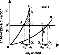
Figure 2. Marginal Abatement Curves Used for Trade Studies.
Table 2. Basics of Trade Studies
| No Trade | Trade between R1 and R2 | |
| Constraints | R1: q1 abated R2: q2 abated |
R1 and R2: q1 + q2 abated |
| Marginal Cost / Market Price | R1:
p1 R2: p2 |
R1
and R2: p' such that p'1(q'1) =
p'2(q'2) = p' and q'1 + q'2 = q1 + q2 |
| Abatement Cost | R1:
area AOQ1 R2: area BOQ2 |
R1:
area (A'OQ'1) R2: area (B'OQ'2) |
| Emission Permits Trading | NA | R1: buys right to emit q1 - q'1 R2: sells right to emit q'2 - q2 = q1 - q'1 |
| Imports (+) / Exports (-) Flows | NA | R1: pays p' x (q1 - q'1) = area (A'I1Q1Q'1) to R2 R2: receives p' x (q'2 - q2) = area (B'I2Q2Q'2) from R1 |
| Total Cost | R1: area AOQ1 R2: area BOQ2 |
R1: area (A'OQ'1) + area (A'I1Q1Q'1) < area (AOQ1) R2: area (B'OQ'2) - area (B'I2Q2Q'2) < area (BOQ2) |
| Savings from Trading | NA | R1:
area (AI1A') (hatched) R2: area (BI2B') (hatched) |
2.3 How Can MACs Be Generated by the EPPA Model?
To build the MACs, we run the EPPA model under different constraints corresponding to different levels of carbon abatement, such as 10%, 20%, or 30% below reference emissions. For each set of constraints, the corresponding, regional shadow prices of carbon are an output of the model. Then we plot the shadow prices as a function of the level of abatement, for time T and region R. A line can then be fitted between the plots to get the MAC of a region R at time T (for example, in the Kyoto case, we are interested in time T = 2010).
As an example, Figure 3 shows the results obtained for the four OECD regions in 2010 when the policies applied are proportional reductions by all OECD regions (1, 5, 10, 15, 20, 30 and 40% of reference 2010 emissions) in 2010, and no reduction by other regions. Here, the shadow prices have been plotted as a function of the percentages of carbon emission reductions (and not the absolute quantities), in order to show the variations across regions without taking into account the size of the economy. We can see that, for any equal percentage reduction, the abatement of the corresponding quantities would cost most in Japan and least in USA and OOE among the OECD regions.
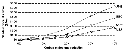
Figure 3. EPPA-Generated Marginal Abatement Curves for 2010. OECD Regions, Proportional Reductions, No Trading.
Similar curves can be obtained for all regions. For example, we can apply the same proportional reductions, but to all of EPPA's twelve regions at the same time.[5] Figure 4 displays the marginal abatement curves thus obtained. It shows where it is the cheapest to abate carbon emissions (India and China) and where it is the most expensive (Japan). To allow trade studies such as illustrated in Fig. 2, we first need to re-scale the x-axis of these curves to actual absolute quantities instead of percentages, which is the way MACs will now be represented.
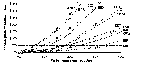
Figure 4. EPPA-Generated Marginal Abatement Curves for 2010.All Regions, Proportional Reductions, No Trading.
2.4 Assessing the `Robustness' of MACs with Regard to the Policy Applied
One question that arises immediately from our use of equal proportional reduction across regions to generate the MACs is whether the location of these curves, or more generally, the cost associated with any given level of carbon abatement, is affected by differing levels of abatement in other regions. For instance, as can be seen in Table 1, the levels of implied abatement corresponding to the Kyoto commitment are not strictly proportional, and with emissions trading, we would not expect the percentage reductions among regions to remain the same. Will region R1's MAC look different depending on whether region R2 reduces by 10% or 40%? In a model with international trade in all goods, such as EPPA, there is the possibility that a 40% reduction by region R2 would alter trade flows such that abatement of, say, 100 Mton by R1 would cost more (or less) than if R2 reduced emissions by only 10%. This fundamental question is that of the robustness of the MACs. And indeed, a drawing like Fig. 2 and the simple method we have deduced from it assume this robustness (one curve for each region, whatever the reductions in other regions). The answer: they are robust.
For example, Figure 5 shows simultaneously the two sets of MACs corresponding to varying levels of OECD abatement assuming no emissions trading and fully efficient emissions trading.[6] The curves in both sets are similar (less than 10% variation in price for any given level of abatement), thus showing that the MACs are robust with regard to this change of policy. We have made similar comparisons for Annex B trading and global trading, and we have examined one region's MAC (the USA) when all other regions vary from reference to as much as a 60% reduction. In all cases, we have found the same fundamental result: whatever the trading scheme, whatever the extent of the market, the marginal abatement curves are almost identical. These model results indicate that abatement cost in a region is largely independent of abatement efforts in other regions.
Our conclusion is that MACs, and more generally, the costs associated with a given level of domestic abatement, are robust to different levels of abatement among regions and the scope of emissions trading. Whatever the reductions of other regions, a MAC for a region R at time T looks the same.
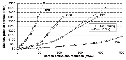
Figure 5. EPPA-Generated Marginal Abatement Curves for 2010. OECD Proportional Reductions, No Trading / OECD Trading.
2.5 Analytical Approximations: A Simple Tool for Trade Studies
Robustness implies that each region at time T has a unique marginal abatement curve. This fundamental result validates the use of marginal abatement curves, and makes actual trade analysis straightforward and simple. Analysis can be simplified even further if each curve could be described by a single mathematical expression because, once we have the equations of the MACs, the cost calculations (i.e. integration under the curves) are extremely simple and rapid.
Figure 6 shows, for the OECD regions, that we can fit simple analytical curves to the sets of plots resulting from the EPPA runs, and that those fits are very good (for each curve, R2 is very close to 1). This result is true for all the other regions as well. The curves that best fit the EPPA-generated plots are of the form: P = aQ2 + bQ, where Q is the amount of abatement in million metric tons of carbon (Mton) and P is the marginal cost, or shadow price, of carbon in 1985 US$. [7] By integration, the total cost of abatement is: C = 1/3 * aQ3 + 1/2 * bQ2). Table 3 displays the coefficients a and b for each region in 2010, as well as the coefficient of determination, R2.
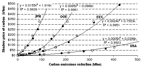
Figure 6. Marginal Abatement Curves for 2010. OECD Regions, Polynomial Approximations.
Table 3. Coefficients of the Approximations of the MACs of the Form: P =
aQ2 + bQ
Region
a
B
R2
Region
a
b
R2
USA
0.0005
0.0398
0.9923
EEX
0.0032
0.3029
0.9983
JPN
0.0155
1.816
0.9938
CHN
0.00007
0.0239
0.9992
EEC
0.0024
0.1503
0.9951
IND
0.0015
0.0787
0.9970
OOE
0.0085
-
0.0986
0.9981
DAE
0.0047
0.3774
0.9996
EET
0.0079
0.0486
0.9973
BRA
0.5612
8.4974
0.9997
FSU
0.0023
0.0042
0.9938
ROW
0.0021
0.0805
0.9967
In using these approximations, analysts should keep in mind that the price of this simplicity is some loss of the details of the general equilibrium features of the underlying model. The robustness of the curves assures us that the relation between price and quantity of abatement is relatively fixed, but the curves do not capture all the effects of emissions trading. Since the EPPA model remains our primary analysis tool, we have run the model in every policy case we studied not only to ensure that the approximations are not misleading, but also to check for any significant side effects. The prices and quantities for abatement were all very close to the approximations, but there is a side effect that the MACs do not show: `leakage.' As will be discussed more extensively later, when only some regions' carbon emissions are constrained, carbon emissions tend to leak to non-constrained regions. Nevertheless, these effects are not essential to the analysis, and the analytical approximations are a powerful computational shortcut to particular results. They provide a convenient way to graphically represent the results of the analysis of trading, and we use them extensively for that purpose in the remaining sections.
2.6 Aggregate Supply and Demand Curves
Marginal abatement curves are the basis for determining the demand and supply for emission permits in any given market. Emission permits represent `rights to emit' and these rights can be produced by some party abating more than it is required to do, or undertaking some abatement when not required to do so. The willingness of any party to purchase or to sell these permits is illustrated by Figure 7. The vertical dotted line represents the amount of abatement required for a region to meet its Kyoto commitment. In the absence of any emissions trading it would abate the amount indicated by the intersection of this line with the MAC, and the corresponding price would be its autarkic marginal cost. If emissions trading were a possibility, the region would purchase or sell permits according to the relation of the market price to its autarkic marginal cost.
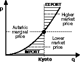
Figure 7. Willingness to Import / Export with Regard to Market Price of Permits.
For whatever market one is considering, we simply add up the quantities (x-axis) potentially supplied and those potentially demanded at each price (y-axis) across the constituent regions. As we vary the price, we describe the demand and the supply curves for this market, and their intersection indicates the market clearing price on the y-axis and the total quantity traded in that market on the x-axis. Examples of aggregate demand and supply curves for the Annex B and global markets will be introduced subsequently.
3. CASE STUDIES OF PERFECTLY COMPETITIVE TRADING
As a first step in illustrating how the cost of meeting Kyoto commitments for different regions is affected by emissions trading, we consider a simple case consisting of only the four OECD regions (USA, JPN, EEC, OOE). We then expand the scope of the market to include all Annex B regions, i.e., OECD + FSU + EET. Finally, to illustrate full global trading, we broaden the market to include the potential supply from the non-Annex B regions. All the numerical results corresponding to different cases are displayed in the tables presented in Section 7.
3.1 A First Case Study: OECD Only
3.1.1 The No-Trading Case
The MACs for the four OECD regions are all presented on Figure 8. The diamonds on the MACs correspond to the quantity of abatement required to meet the Kyoto commitment for each region, on the horizontal axis, and, on the vertical axis, the no-trading, or autarkic, marginal cost for that region. The autarkic marginal cost of abatement for Japan ($584/ton) is much higher than the marginal costs of abatement for the EEC ($273), the OOE ($233), or the USA ($186). The areas under the curves represent the total costs of abatement for each region. The total cost for the OECD is $115 billion.
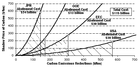
Figure 8. OECD Regions Meeting their Kyoto Commitment, No Trading. (Table A)
3.1.2 The Trading Case
Figure 9 depicts what happens when there is emissions trading. Regional marginal costs equalize in such a way that the total amount of carbon abated is the same as in the no-trading case (the arrows on the x-axis, which represent the changes in quantities of carbon abated when trade occurs, sum to zero). The resulting price is the market price of emissions permits ($240/ton). It is below the autarkic marginal costs for JPN and the EEC, but above those for the OOE and USA. Consequently, JPN and EEC are importers of permits equivalent to 86 Mton of higher-cost domestic abatement avoided, while the OOE and USA undertake additional abatement in this amount to export the permits. Every region achieves some gains through trading, and the total savings for the OECD are $13 billion. The areas representing the regional savings from trade are displayed as the hatched areas on the graph for JPN and USA. Japan imports the most, 65 Mton i.e. 45% of the reduction required by its Kyoto commitment, and benefits the most from emissions trading ($10 billion). The USA is the principal exporter (83 Mton) and it draws the second largest benefit from emissions trading in this market ($2 billion). The EEC imports and the OOE exports smaller amounts of emission reductions, respectively, and each benefits by less than $1 billion. These relationships point out an important feature of emissions trading: regions whose autarkic marginal cost is farther from the trading equilibrium will import (or export) more and benefit more than those regions whose autarkic marginal cost is closer to the trading equilibrium.
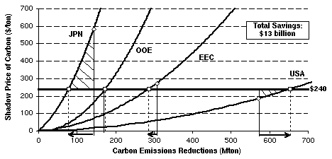
Figure 9. OECD Regions Meeting their Kyoto Commitment, No Trading/Trading. (Table B)
3.2 Trading with All Annex B Regions
3.2.1 No Trade / Trade within Annex B Regions
Here we conduct the same analysis as above, except that the FSU and EET are included. In the no-trading case, the marginal cost of meeting the Kyoto commitment for the EET is $116/ton and its total cost of abatement is $5 billion. As for FSU, the commitment made at Kyoto would not result in a constraint on its carbon emissions, according to our model and nearly all predictions, because its Kyoto commitment corresponds to an emission level higher than the one predicted for 2010 (see Table 1). Therefore, compliance with Kyoto would result in no cost whatsoever for the FSU. The cost of compliance for all of Annex B would be $120 billion, i.e. the $115 billion for OECD regions, + $5 billion for EET.
In the emissions trading case with the FSU and EET included, the equilibrium market price is much lower than in the OECD only case, $127/ton. The OECD regions are all importers of permits, since the market price is lower than autarkic marginal cost for all of these regions; and the EET and FSU are exporters. The FSU accounts for virtually all of the exports (98%). As shown in Figure 10, about a third of these consist of `hot air,' with a cost of zero; but the remaining exports are generated by abatement undertaken to earn additional export profits up to the point that marginal abatement cost equals the market price. It costs the FSU $10 billion to abate the 234 megatons (Mton), but the permits can be sold for $30 billion for a net gain of $20 billion. When added to the $14 billion earned for exporting 111 Mton of the unused Kyoto entitlement, the FSU's total gain from emissions trading is $34 billion.
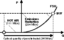
Figure 10. Trade with FSU: The `Hot Air' Effect.
For the five Kyoto-constrained regions, the cost of meeting the Kyoto commitment is reduced by $32 billion, as illustrated in Figure 11.[8] The four OECD regions avoid more costly domestic abatement by importing permits, and the EET is able to reduce its costs by a small profit on its exported permits. The reductions in cost, that is, the gains from emissions trading for the five Kyoto-constrained regions, are distributed roughly in proportion to autarkic marginal cost. The two regions with the highest autarkic marginal costs, Japan and the EEC, benefit the most from emissions trading in this market. Japan imports 66% of its reduction requirement and reduces its cost by $19 billion. The EEC imports 35% of its reduction requirement and reduces its cost by $7 billion. These two regions account for about one-third of the total emission reduction requirement for the five Kyoto-constrained regions, and about five-sixths of the gains from emissions trading for these regions accrue to them. The other three regions are characterized by autarkic marginal costs much closer to the Annex B market price; consequently, they trade much less. The USA and OOE are importers for 19% and 25% of their respective requirements, and the EET abates emissions by 5% more than required in order to export permits. The gains for these regions, which account for two-thirds of the total reduction requirement, total $5 billion, about a sixth of the gains from trading for the Kyoto-constrained regions. From the standpoint of world resource use, the aggregate cost of meeting the Kyoto commitments is much lower with Annex B trade ($54 billion) than without ($120 billion). The total gains from emissions trading are $66 billion, split about evenly between the FSU ($34 billion) and the OECD + EET ($32 billion).
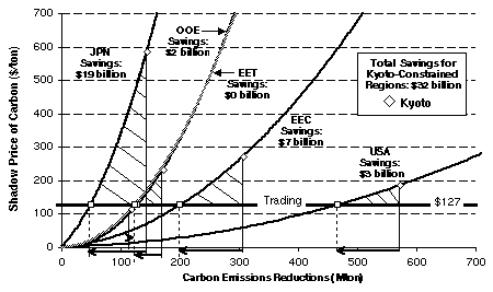
Figure 11. Annex B Meeting their Kyoto Commitment, No Trading/Trading. (Tables C & D)
3.2.2 How Much Difference Does the `Hot Air' Make?
Part of the gains from Annex B trading results from a controversial feature that has come to be called `hot air:' the difference between the FSU commitment at Kyoto and its predicted emissions level in 2010. Since no abatement is undertaken to produce these permits, their export relaxes the aggregate constraint faced by the five Kyoto-constrained regions by about 8%. As a result, many observers argue that such exports should not be permitted, although admittedly, were the FSU's economy to grow faster than predicted here, global emissions would rise equivalently. From this point of view, the FSU's commitment represents a permissible level of emissions, which if unused is available for banking or export, as would be the case for any other Annex B party.
It is possible, of course, to model Annex B trading without the `hot air,' i.e. without allowing the FSU to sell permits that do not correspond to actual emission reductions.[9] With less supply, the Annex B market clearing price is higher, $150, so that the OECD regions + EET abate 90 Mton more domestically, import correspondingly fewer permits, and pay more for those imports (Table E). At this higher price, the FSU also abates more (20 Mton) and it sells 90 Mton less, hence 254 Mton. It is interesting to note that the reduction in the gains from trade are shared about equally: $9 billion less for the FSU (-25%) and $7 billion less for the OECD + EET (-21%).
Nevertheless, the reduction in OECD compliance cost and the corresponding gains from emissions trading, $51 billion, are still substantial and much greater than if trading were restricted to OECD regions only. This result occurs because, so long as the FSU is not as severely constrained by a Kyoto commitment as its potential trading partners are, it remains a very cheap source of emission reductions.
3.3 Full Global Trading
3.3.1 Adding the Non-Annex B Regions
To illustrate full global trading, we rely on aggregate supply and demand curves for emissions permits, as explained earlier and now illustrated in Figure 12. These curves indicate the total quantities of permits that would be supplied or demanded at various price levels in a given market. In the figure, there is only one demand curve because the Kyoto-constrained regions are the same in both the Annex B and the global markets. This single demand curve intersects the horizontal axis at the quantity equal to the sum of the emission reductions required to meet the Kyoto commitments, 1.31 Gton. This is the `Kyoto cap' represented by a vertical dotted line on the figure; it is also the quantity of emission permits that would be demanded if the price were $0/ton. At this price, the aggregate supply is the quantity of permits available at no cost: the FSU's `hot air,' 111 Mton.
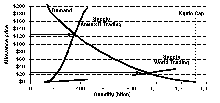
Figure 12. Aggregated Supply and Demand Curves in 2010 under Kytoo Constraints. Annex B Trading / World Trading. (Table F)
As the price increases, the demand for permits diminishes, as more and more domestic abatement is undertaken, and the supply of permits increases as more abatement is justified in the exporting regions. As long as the market price is less than $116, the lowest autarkic marginal cost for the Kyoto-constrained regions,[10] these regions are always on the demand side; and the unconstrained regions are on the supply side. When the price reaches the marginal cost for EET, $116, this region becomes an exporter, supply grows faster, and the demand decreases more slowly, resulting in a `kink' on all curves, which is almost indiscernible because of the EET's small economic size. Such a kink is, however, readily seen on both supply and demand curves when the price reaches $186, the autarkic marginal cost for USA. There will be similar kinks at $233 when OOE becomes a supplier and at $273 when the EEC does. At $584, the autarkic marginal cost for Japan meeting the commitment, the demand for permits will be zero.
The ample supply of permits from non-Annex B regions causes a marked shift in the supply curve and results in a market price that is much lower ($24/ton) than in the Annex B trading case. The total cost of reducing global CO2 emissions to achieve the Kyoto goals is astonishingly low: $11 billion vs. $54 billion with Annex B trading or $120 billion with no emissions trading!
At this price, the Kyoto-constrained regions depend far more on imports than when trading was restricted to Annex B regions only. In the aggregate, 71% of OECD + EET commitments are met through importing emission reductions from non-constrained regions; and the largest importers (proportionately) are those regions facing the highest autarkic marginal cost: Japan, 92%; EEC, 76%; USA, 68%; OOE, 66% and EET, 56%. On the suppliers' side, three countries account for the bulk of exports: China (47%), the FSU (23%) and India (11%), hence 81% altogether. Whether because of relatively small size or high relative abatement costs, the remaining four non-Annex B regions are small suppliers of emission permits to the Annex B regions.
With full global trading, the gains from emissions trading are much greater for the Kyoto-constrained regions ($94 billion vs. $32 billion with Annex B trading). The non-Annex B regions gain $10 billion by exporting permits, but their gains are much less than those of the Kyoto-constrained regions. The FSU is the only party that is worse off by this widening of the market. At $24/ton, the FSU abates about half as much as before, (101 Mton), and the `hot air' is worth much less. As a result, the FSU's net gain ($4 billion) in the global market is much less than when it does not compete with the non-Annex B regions ($34 billion). The distribution of the gains from emissions trading in the global market illustrates again the feature of emissions trading we just noted: regions whose autarkic marginal cost is further from the equilibrium price benefit more than regions whose marginal cost is closer to that price: in this global trading case, the clearing price is much closer to the shadow price of the exporting regions when they are not involved ($0/ton) than it is to the autarkic marginal cost of any of the importers.
3.3.2 Hot Air and Leakage
One of the arguments surrounding the use of emissions trading has been that it would increase global emissions, unless the `hot air' from the FSU (or elsewhere) could be kept out of the system. This argument ignores an interesting feature of the general equilibrium solution of CGE models, to which we alluded earlier: leakage. When only a sub-set of the regions of the world are constrained and there is no emissions trading, emissions `leak' to unconstrained regions; however, with emissions trading, there is no leakage, since all regions face the same carbon price.
The compensating effects of leakage and hot air are shown in Figure 13. If there were no leakage and no hot air, the 1,312 Mton reduction of emissions required of the five Kyoto-constrained regions could be expected to reduce 2010 global emissions from 9,098 Mton to 7,786 Mton. In the no trading case, a total 62 Mton of leakage (10 Mton to the FSU and 52 Mton to the non-Annex B regions) offsets a portion of the Annex B emission reduction, so that global emissions are actually 7,848 Mton. When the FSU is included in the trading regime, there is no leakage to the FSU since the carbon price is the same as in the Kyoto-constrained regions, but there is still some leakage to the non-Annex B regions. This amount is less, 35 Mton, because the price attached to carbon, and thus the incentive to leak, is less for all the Kyoto-constrained regions.[11] Global emissions increase not by 111 Mton, the amount of hot air, but by 84 Mton (111 Mton less the reduction in leakage, 27 Mton). With full global trading, there is no leakage whatsoever, as all regions face the same carbon price, and the net increase in global emissions associated with emissions trading is only 48 Mton.
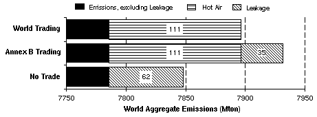
Figure 13. Actual Levels of Emissions in the Different Trading Cases: Effects of Leakage and the FSU `Hot Air.' (Table G)
The particular numbers obtained in this model simulation are not what should be stressed. The important point is that, when evaluating emissions trading, the effect of `hot air' on the global reduction of emissions cannot be considered in isolation from leakage. Emissions trading would allow `hot air' into the system to the extent any party's Kyoto commitment is not binding, but it also reduces leakage to countries with non-binding commitments or no commitment at all. The net balance depends upon the amount of leakage and hot air, and both are sensitive to the model's emission prediction for countries with non-binding Kyoto commitments and its specification of the trade sector. For instance, higher 2010 emissions for the FSU will reduce hot air without much effect on leakage, and more substitutability in trade will lead to more leakage. Other assumptions than those presented here could easily yield results that would indicate that emissions trading would lead to a net reduction of global emissions. In sum, the interaction of leakage and emissions trading calls for a more nuanced treatment of `hot air.'
3.4 Summary of the Three Competitive Trading Cases
Figures 14 and 15 summarize the three competitive cases we have studied: no trade; trade within Annex B; and world trade, with respect to both the quantity and cost aspects of meeting the Kyoto commitments.
In Figure 14, the five constrained Annex B regions are represented by bars extending to the right representing the combination of domestic abatement and imported permits that would be chosen by each of these regions to meet the Kyoto commitment. For the two trading cases, the darker portions indicate the amount of the commitment met by importing emissions permits, and the percentage of imports is indicated. The quantities imported are progressively larger as the scope of the market is expanded (from bottom to top for each region) to include more low cost sources of emission reduction. The exporting regions--FSU and non-Annex B, and EET in the Annex B trading case--have bars both to the right and to the left. The amount of emissions reduction they undertake is indicated to the right; and to the left, the amount of emissions permits they export.[12] Those amounts are equal, except that the FSU disposes of a quantity of permits it can sell without undertaking any reductions, namely, the `hot air,' represented by the cross-hatched segment of the bar. This `hot air' shows up on the right-hand side in the smaller quantities of reduction associated with the two trading cases for Annex B and the World.
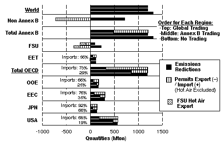
Figure 14. The effects of Trading: Emissions Reductions, Trade Quantities, Hot Air.
Figure 15 compares the effects of the Kyoto commitment, across cases, in terms of costs, that is, the quantities of Fig. 14 multiplied by prices. While trading benefits every region to some extent, two points become quite clear from this graph. First, the Kyoto-constrained regions facing relatively higher marginal costs derive relatively greater benefit from emissions trading. In both trading cases, Japan and the EEC import more and benefit more than does the USA, because the latter faces lower marginal costs of meeting the Kyoto commitment than the other regions. Second, the FSU exports more and benefits more when it does not compete with the non-Annex B regions to satisfy the demand from the importing regions. Notably, it is the only region that fails to gain from the expansion of the market to embrace global trading, and its loss is striking.
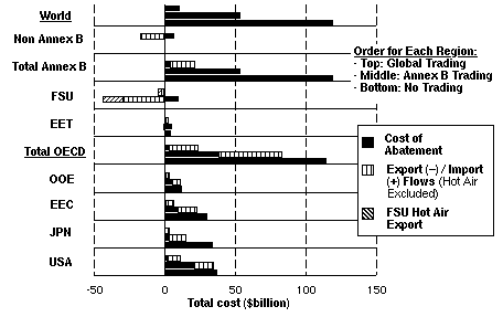
Figure 15. The Effects of Trading: Regional Abatement Costs and Trade Flows.
4. DEPARTURES FROM PERFECT TRADING
All of the cases studied so far assume that potential participants in emissions trading are not impeded by restrictions on trading, that competitive conditions apply, and that trading is conducted efficiently with low or non-existent transactions cost. Such assumptions simplify the analysis and exposition of emissions trading, but they are not necessarily realistic. In this section, we use the aggregate demand and supply curves to evaluate the effects of departures from these simplifying assumptions.
4.1 The Effect of Quantitative Limits on Demand
The Kyoto Protocol itself contains provisions relating to `supplementarity' that suggest that a party's ability to rely on emissions trading for meeting its Kyoto commitment may be limited in some manner. This provision has been given further impetus by the call for a "concrete ceiling" by the EU environmental ministers. The imposition of a limit on imports would affect the gains from trade; and in this section, we illustrate the effects by assuming a limit of 33% on any Annex B party's ability to meet its emission reduction requirement through imported permits.[13]
In the case of Annex B trading without restrictions, Japan would optimally realize 66% of its Kyoto commitment through imports, well above the 33% limitation, and EEC 35%, slightly above the limit, while none of the other importing regions would be constrained. As a result, Japan would import commensurately fewer permits and have to abate more domestically, up to a marginal cost of $322/ton. However, this is not all that happens.
As illustrated in Figure 16, less demand shifts the aggregate demand curve downwards, so the market clearing price is slightly lower than it otherwise would be: $114/ton. As an interesting result, all the regions that are not affected by this limit import more in response to the cheaper price, and they reduce domestic abatement by a corresponding amount. The USA would thus increase permit imports from 19% to 23% of its emissions reduction requirement, OOE from 25% to 29%. Those regions are unambiguously better off because the supplementarity condition removes the potential demand by higher cost abaters from the emissions trading market. Japan accrues some benefit from the cheaper permit imports, but the savings are swamped by the higher costs for significantly more domestic abatement.[14] EEC imports also are affected by the limit, but it benefits slightly from the lower price for the permits it does import. Overall, on the importers' side, the aggregate savings is practically the same, (99% of that of the non constrained case), but the gains are redistributed, mostly from Japan that loses $4 billion of potential gains, to USA, EEC, OOE. The two exporters, the FSU and EET, are hurt as well. The FSU sells slightly fewer permits at a lower price, thus losing $4 billion of potential gains. EET's gains as an exporter disappear, as it becomes a small importer. Overall, the aggregate gains from emissions trading are only reduced from $66 billion to $61 billion.
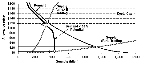
Figure 16. Annex B / World Supply and Demand in 2010 under Kyoto Constraints. Demand from Each Importing Region Limited to 33% of Commitment. (Tables H & I)
The exact numbers and effects will vary of course depending on the supplementarity limit and on the reduction required of various parties to meet the Kyoto commitment. The essential feature is that while the global costs might be a little higher with the supplementarity constraint, such a restriction on imports affects countries very differently. As a result, there is a significant redistribution of gains within importing regions, from regions with relatively high abatement cost, who would otherwise depend more heavily on imports, to regions with relatively low abatement cost.
The same 33% limit on imported permits would have a much greater effect with full global trading. Now, all the importing regions are constrained by the limitation. The price of imports is much lower than in the unconstrained case, $6 vs. $24, but for the constrained regions, the cheaper imports do not make up for the higher domestic abatement cost required: all importing regions, except EET, are worse off. Thus, for the OECD + EET, the aggregate cost for meeting the Kyoto commitments rises from $26 billion to $43 billion. The exporting regions gain virtually nothing in this situation ($1.7 billion compared to the $14 billion possible gains in the unconstrained situation), because of the restricted demand and the very low market price.
4.2 Non-Competitive Behavior in Supply
It is premature to worry about non-competitive behavior in a market that is not yet created, but there are dominant suppliers in each of the markets we have reviewed and we have examined the gains from emissions trading only under the assumption that maximizes those gains: perfect competition. The FSU is a particularly dominant supplier in the Annex B market and we turn to that case first.
4.2.1 The FSU in the Annex B Market
As an unconstrained Annex B region with hot air, the FSU is the source of the significant gains associated with Annex B trading and the almost exclusive supplier of permits in this market. The FSU is no longer a single political entity, but for the sake of illustration we show what would be the effect if the constituent nations were to take advantage of their dominant position by colluding to limit supply in order to maximize their profit.[15] The effect is not great: the price of permits is raised slightly, to $142/ton vs. $127 in the competitive case (Table J). The reason is that, as the price rises, the importing regions abate more and import less. It makes sense for the FSU (or any monopolist) to restrict supply only so long as the increase in price more than compensates for the decrease in quantity exported. In this case, the elasticity of the aggregate demand curve is such that there is not much to gain for the FSU by restricting supply. As a result, the gains from emissions trading are only slightly less than in the competitive case ($64 billion). What is changed is the distribution of the gains from emissions trading. The FSU increases its gains by $2.4 billion, while the gains for the importing regions is diminished by $4.7 billion. The benefits from emissions trading for the importing regions are still significantly greater than when there is no trading.
4.2.2 A Non-Annex B Cartel?
In full global trading, there is no dominant supplier of permits; however, the Kyoto Protocol does specify that non-Annex B emission reductions are to be provided to Annex B parties through a Clean Development Mechanism (CDM). The role of the CDM is not yet established; however, part of the rationale for it appears to be ensuring that non-Annex B countries receive acceptable prices (however determined) for their permit exports.[16] And indeed, as shown earlier, the prices under full global trading would be very low, compared to other alternatives. Furthermore, at a price of $24 and a volume of trade of 935 Mton of emissions reductions, elasticity conditions are more favorable to collusive behavior than in the Annex B case. Nevertheless, assuming successful combination through the CDM or other means, the non-Annex B nations do not enjoy as dominant a position as the FSU in the Annex B market. As a group, the non-Annex B regions supply 77% of the permits in full global trading, whereas FSU supplies 98% in the Annex B market. Consequently, any attempt by the non-Annex B regions to restrict supply would have to take into account the response of the FSU. We study below two cases: FSU competing with the non-Annex B regions and FSU cooperating.
In the first case, only the non-Annex B regions are acting as a monopoly.[17] The Annex B regions are all price takers, OECD + EET as importers, and the FSU as an exporter. The market price is significantly increased (to $63), so that the importers abate more and import 279 Mton less (Table K). Their gains from global emissions trading are reduced from $94 billion to $59 billion. Non-Annex B regions more than double their gains (now $22 billion) despite the reduction in exports by 342 Mton. As a competitive supplier, the FSU benefits doubly, from the higher price and greater exports (+63 Mton). Its gains from trading more than triple, to $14 billion. Overall, the global cost of meeting the commitment is still very low, $20 billion, but the gains from trade have shifted somewhat more in favor of the exporting regions (38% vs. 13%).
When the FSU cooperates with the non-Annex B regions, the resulting price, $108/ton, is considerably higher (Table L). What happens in the first case is here enhanced: the gains from emissions trading to the importing regions are reduced another $24 billion, to $34 billion, while those to the suppliers are increased, by $4 billion for the FSU and by $8 billion for the non-Annex B regions. Both the non-Annex B regions and the FSU cut back exports drastically compared to the fully competitive case, -24% for FSU, to 161 Mton, and -61% for non-Annex B regions, to 285 Mton. [18] The overall gains from trade are reduced to $82 billion, which is still considerable, and shifted even more in favor of the exporters (58% of the total gains). This case, the best possible one for the suppliers, provides the theoretical limit of the suppliers' gains from trading emissions permits in a world market: $47 billion.
These two cases illustrate that, if it could be organized, there is ample room for non-competitive behavior in the global emissions trading market, in contrast to the Annex B market. Such behavior leads to significant redistribution of the gains from importing regions to exporting regions, whether the FSU competes or cooperates with the non-Annex B regions. Furthermore, the gains to importing regions from emissions trading would still be very large, and greater than would be the case if trading were restricted to the Annex B regions only. For the FSU however, the gains would remain always lower than in the Annex B trading case.
4.3 Transactions Cost and Other Inefficiencies in Supply
A far more likely outcome in the global market, or the Annex B market for that matter, is that supply would be limited by transaction costs or a more general failure to take advantage of the economic opportunities provided by emissions trading. For instance, concerns about `additionality' and the inherent difficulty of identifying a counterfactual baseline for joint implementation projects may impose high transaction costs and thereby limit the supply from non-Annex B regions.[19] Alternatively, potential suppliers may not pursue available export opportunities with the complete economic rationality assumed by EPPA. Such departures from the model's assumptions can be easily simulated by assuming that only a certain share of what is potentially available at any given price would be supplied. If such were the case, the aggregate supply curves would be shifted upward and the market clearing prices would be higher, as shown in Figures 17 and 18.
Figure 17 illustrates the effect of a 50% reduction in available supply from the FSU due to such imperfections, in the Annex B trading case, assuming unfettered demand.[20] The price is raised to $167/ton, compared to $127 when completely efficient supply is assumed. As a result, the role of EET as a supplier in increased (to 11% total), as well as its benefits. Importing countries whose autarkic marginal cost is low, such as the USA, almost do not resort to trade, hence their gains decrease, while emissions trading still conveys considerable benefits to the relatively high cost abaters, Japan and the EEC. The FSU exports fewer permits than otherwise (now 190 Mton compared to 345 Mton), but at a higher price, so it still benefits from this new export opportunity, although its gains are reduced, to $30 billion from $34 billion.[21] The gains from emissions trading are less for all parties, but at $51 billion in the aggregate, those gains are still important.
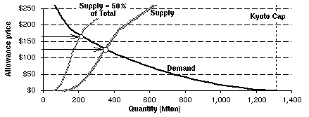
Figure 17. Annex B Permit Supply and Demand in 2010 under Kyoto Constraints. Inefficient Supply: Supply = 50% Total. (Table M)
Figure 18 depicts the market equilibrium when only 50% and 25% of the quantities available from the FSU and non-Annex B regions are available. As was the case with Annex B trading, the price increases with the reduced supply, from $24 to $52 and $94 respectively. As before, the gains from trade for the importers are less than otherwise, especially for the low cost abaters, but still appreciable. The interesting feature is what happens on the supply side. Unlike the case with Annex B trading with such imperfections, the gains to the supplying regions are enhanced. The increase in the price more than compensates for their limited ability to supply, and their gains are significantly increased (+85% and +137% respectively for non-Annex B regions, +30% and +35% respectively for FSU).[22]
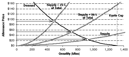
Figure 18. World Permit Supply and Demand in 2010 under Kyoto Constraints. Inefficient Supply: Supply = 50% and 25% of Total. (Table O)
5. CONCLUSIONS
5.1 A Readily Available Technique for Analyzing Trading Issues
Emissions trading raises many issues concerning magnitude and distribution of the benefits from trade. The primary purpose of this paper has been to explain a readily available technique for analyzing and explaining these issues. Marginal abatement curves are often drawn illustratively, but for all their heuristic value, good empirical estimates of these curves are hard to find. The MACs used here are not empirically estimated, but they are derived from the complex economic models that are commonly used to predict emissions and to evaluate the costs of various policies. As such, they are a compromise: better than purely heuristic curves, but not as good as an empirically estimated relationship. They are in fact only as good as the underlying models, which, for all their faults, are still commonly relied upon to provide insight and estimates of costs and other effects. Analysts who lack such a model and who have a slight aptitude for algebra can take the parameter estimates provided in Table 3 and conduct their own analyses.
It can also be hoped that other modeling groups will make explicit the MACs that are generated by their models, so that policy analysts will have the benefit of knowing how alternative representations of the underlying economic reality will affect the magnitude and distribution of the gains from emissions trading.
5.2 Emission Permit Trading: Implications for Policy
The object of any analytic exercise is to gain insight into policy issues; and many arise from this exercise.
The most fundamental is almost trivial: any emissions trading, no matter how constrained or imperfect, is better than none at all. The effect of trading is always to require less resources to achieve the same environmental goal, and thereby to preserve resources for other useful social goals. There is no emissions trading scheme in which all participating parties do not derive at least some benefit.
Second, the potential for gains from trading is huge, because of the considerable differences in abatement costs across regions. This potential should certainly provide incentives to both Kyoto-constrained and unconstrained regions to support emissions trading.
Third, from the standpoint of husbanding the world's limited resources, the fewer the constraints on trading the better. Even though non-competitive behavior and other departures from perfect trading do not eliminate the gains from emissions trading, they do inevitably increase costs.
Fourth, the gains from emissions trading will not be evenly distributed. As a general rule, regions whose autarkic marginal cost of abatement is relatively far from the market price of permits for a given market will derive the greatest benefit from emissions trading.
Fifth, unlike all other regions, the FSU is adversely affected by opening the market to non-Annex B supply. The potential conflict of interest between the FSU and non-Annex B regions may influence future negotiations over accession to Annex B or expanding trading to non-Annex B nations.
Finally, limitations and imperfections not only reduce the overall gains from trading, they also redistribute the remaining gains, often in unsuspected ways. For instance, a quantitative limitation on imports reduces the gains from emissions trading for exporters and for countries whose imports are restricted; but it benefits importing countries that are not affected by the limitation. Also, transaction costs and other forms of inefficiency might be expected to reduce the gains from trading for suppliers; but when supply is ample and prices low, any increase of price increases export revenues and gains from trading, whether due to strategic behavior or plain inefficiency.
5.3 Suggestions for Future Research
Our analysis has been limited to CO2, yet another important dimension of the flexibility accepted at Kyoto is inclusion of the enhancement of sinks and the reduction of other greenhouse gases in meeting Kyoto commitments. Thus, another dimension for further research is broadening of the potential market by the inclusion of sinks and other greenhouse gases. Given appropriate CO2-equivalence, analogous marginal cost curves could be constructed for the enhancement of sinks and the reduction of other greenhouse gases, and any region's resort to CO2 emission reduction, sink enhancement and other GHG emission reduction could be explored using these curves. While aggregate costs would undoubtedly be reduced, it is quite unlikely that the distribution of the gains from trading would be the same as when only carbon is included.
Little has been said about uncertainty, and the analysis presented here is based upon one view of the future, that represented by the reference run in EPPA version 2.6. Other futures are quite possible, and it is evident that the marginal costs faced by Annex B parties in 2010 depend as much upon such predictions of economic and emissions growth as they do upon the relative positions of the MACs or the commitments undertaken at Kyoto. Higher or lower emissions growth may not shift the MACs (as opposed to moving along them), but such variations in growth will certainly affect regional supply and demand for permits, and thus the market clearing prices and trade flows detailed above. An important further research direction is the extent to which the conclusions drawn from this single forecast would be modified by a richer treatment of uncertainty.
The relative position of the MACs constitutes the backbone of this analysis. The MACs generated from EPPA are robust with respect to emissions trading policies and to variations in emissions growth, but we doubt that this result would hold for variations in more fundamental assumptions such as technology and substitution elasticities. The relative positioning of the MACs in EPPA--e.g., Japan as the highest cost abater, EEC next then USA and OOE--seems plausible, but what makes costs in Japan twice as high as in the EEC? And what makes China such a low cost supplier of emission reductions? We have tried to make our conclusions general, and thus not overly dependent on the particular MACs generated by EPPA 2.6; but the practical interest of most policy-makers will remain the application of the general principles to specific countries and regions. This calls for a better appreciation of what underlying characteristics make certain countries relatively high or low cost sources of abatement.
6. ACKNOWLEDGMENTS
We are greatly indebted to many colleagues and associates for consistent encouragement and critical comment. Foremost among these are the faculty and research staff associated with MIT's Joint Program on the Science and Policy of Global Change, particularly the EPPA Working Group. Particular thanks are due to Henry Jacoby, Dick Eckaus, Loren Cox and David Reiner for their careful comments on earlier drafts of this paper and to Ian Sue Wing for invaluable help in running the model. The encouraging response of participants of the Royal Institute for International Affairs (RIIA)/MIT Global Change Forum, held at London in June, 1998, gave much direction to the paper; and we are grateful to Nathalie Kosciusko-Morizet, Jean-Charles Hourcade, Thierry Le Pesant and Ken Chomitz for their subsequent interest and helpful comment. Finally, this research would not have been possible without the funding made available to the Joint Program by a number of corporations in the U.S., Europe and Japan, by EPRI, and by agencies of the Norwegian and U.S. Governments.
All the prices in the following tables are in 1985$.
NAB = Non-Annex B regions
TABLE A: Kyoto OECD only no trading
| USA | JPN | EEC | OOE | OECD | |
| Reductions / ref 2010 (Mton) | 572 | 144 | 307 | 171 | 1194 |
| Marginal Costs ($/ton) | $186 | $584 | $273 | $233 | \ |
| Cost of Abatement ($billion) | 37.62 | 34.37 | 30.29 | 12.81 | 115.09 |
TABLE B: Kyoto OECD only OECD trading
USA
JPN
EEC
OOE
OECD
Reductions / ref 2010 (Mton)
655
79
287
174
1194
Market Price of Permits ($/ton)
$240
$240
$240
$240
$240
Cost of Abatement ($billion)
55.28
8.22
25.02
13.44
101.96
Permits exp(-)/imp(+) (Mton)
-83
65
21
-3
0
i.e
% of commitment (import)
\
45%
7%
\
\
Flows
exp(-)/imp(+) ($billion)
-19.95
15.66
4.94
-0.64
0.01
Total Cost ($billion)
35.33
23.88
29.96
12.80
101.97
Gains from trade ($billion)
2.30
10.49
0.33
0.01
13.12
TABLE C: Kyoto no trading
USA
JPN
EEC
OOE
EET
OECD+EET
FSU
World
Reductions / ref 2010 (Mton)
572
144
307
171
118
1312
0
1312
Marginal Costs ($/ton)
$186
$584
$273
$233
$116
\
\
\
Cost of Abatement ($billion)
37.62
34.37
30.29
12.81
4.67
119.76
0.00
119.76
TABLE D: Annex B trading
USA
JPN
EEC
OOE
EET
OECD+EET
FSU
World
Reductions / ref 2010 (Mton)
466
49
201
128
124
968
234
1202
`Hot air' (Mton)
\
\
\
\
\
0
111
111
Market Price of Permits ($/ton)
$127
$127
$127
$127
$127
$127
$127
$127
Cost of Abatement ($billion)
21.16
2.82
9.51
5.16
5.36
44.01
9.95
53.96
Permits exp(-)/imp(+) (Mton)
106
95
106
43
-6
345
-345
0
i.e % of commitment (import)
19%
66%
35%
25%
\
26%
\
\
Flows exp(-)/imp(+) ($billion)
13.44
12.06
13.51
5.49
-0.73
43.77
-43.77
0.00
Total Cost ($billion)
34.60
14.88
23.02
10.64
4.64
87.78
-33.82
53.96
Gains from trade ($billion)
3.03
19.49
7.27
2.17
0.03
31.99
33.82
65.81
TABLE E: Annex B trading, No hot air
USA
JPN
EEC
OOE
EET
OECD+EET
FSU
World
Reductions / ref 2010 (Mton)
509
56
220
139
135
1058
254
1312
`Hot air' (Mton)
\
\
\
\
\
0
0
0
Market Price of Permits ($/ton)
$150
$150
$150
$150
$150
$150
$150
$150
Cost of Abatement ($billion)
27.10
3.73
12.21
6.60
6.86
56.51
12.73
69.23
Permits exp(-)/imp(+) (Mton)
63
88
87
33
-17
254
-254
0
i.e % of commitment (import)
11%
61%
28%
19%
\
19%
\
\
Flows exp(-)/imp(+) ($billion)
9.40
13.23
13.00
4.90
-2.48
38.05
-38.05
0.00
Total Cost ($billion)
36.50
16.96
25.21
11.50
4.38
94.55
-25.32
69.23
Gains from trade ($billion)
1.12
17.41
5.08
1.31
0.29
25.21
25.32
50.53
TABLE F: World trading
USA
JPN
EEC
OOE
EET
OECD+EET
FSU
NAB
World
Reductions / ref 2010 (Mton)
182
12
73
59
52
378
101
723
1202
`Hot air' (Mton)
\
\
\
\
\
0
111
0
111
Market Price of Permits ($/ton)
$24
$24
$24
$24
$24
$24
$24
$24
$24
Cost of Abatement ($billion)
1.66
0.14
0.71
0.41
0.43
3.36
0.81
6.99
11.15
Permits exp(-)/imp(+) (Mton)
390
132
234
112
66
935
-211
-723
0
i.e % of commitment (import)
68%
92%
76%
66%
56%
71%
\
\
\
Flows exp(-)/imp(+) ($billion)
9.27
3.15
5.57
2.67
1.57
22.24
-5.03
-17.21
0.00
Total Cost ($billion)
10.94
3.29
6.29
3.09
2.01
25.60
-4.22
-10.22
11.15
Gains from trade ($billion)
26.69
31.08
24.00
9.73
2.66
94.16
4.22
10.22
108.61
CONTINUED--TABLE F: World trading
EEX
CHN
IND
DAE
BRA
ROW
Reductions / ref 2010 (Mton)
51
437
102
42
2
89
`Hot air' (Mton)
\
\
\
\
\
\
Market Price of Permits ($/ton)
$24
$24
$24
$24
$24
$24
Cost of Abatement ($billion)
0.54
4.22
0.95
0.44
0.03
0.81
Permits exp(-)/imp(+) (Mton)
-51
-437
-102
-42
-2
-89
i.e % of commitment (import)
\
\
\
\
\
\
Flows exp(-)/imp(+) ($billion)
-1.21
-10.40
-2.44
-0.99
-0.06
-2.12
Total Cost ($billion)
-0.68
-6.17
-1.49
-0.55
-0.03
-1.31
Gains from trade ($billion)
0.68
6.17
1.49
0.55
0.03
1.31
TABLE G: Leakage
USA
JPN
EEC
OOE
EET
OECD+EET
FSU
NAB
World
Ref emissions 2010 (Mton)
1838
424
1064
472
395
4193
763
4142
9098
Emissions no trading (MT)
1267
280
757
301
277
2881
773
4194
7848
Reductions / ref 2010 (Mton)
572
144
307
171
118
1312
\
0
1312
Leakage / ref 2010 (Mton)
\
\
\
\
\
0
-10
-52
-62
Emissions Annex B trading (MT)
1353
379
863
341
274
3210
544
4177
7931
Reductions / ref 2010 (Mton)
485
46
200
131
121
983
219
0
1202
`Hot air' (Mton)
\
\
\
\
\
0
111
111
221
Leakage / ref 2010 (Mton)
\
\
\
\
\
0
\
-35
-35
Permits exp(-)/imp(+) (Mton)
87
99
107
40
-3
330
-330
0
0
Emissions World trading (MT)
1637
414
997
414
351
3813
681
3402
7896
Reductions / ref 2010 (Mton)
201
11
66
58
44
380
82
740
1202
`Hot air' (Mton)
\
\
\
\
\
0
111
0
111
Leakage / ref 2010 (Mton)
\
\
\
\
\
0
\
0
0
Permits exp(-)/imp(+) (Mton)
370
134
241
114
74
933
-193
-740
0
CONTINUED--TABLE G: Leakage
EEX
CHN
IND
DAE
BRA
ROW
Ref
emissions 2010 (Mton)
927
1792
486
308
97
532
Emissions
no trading (MT)
940
1801
486
309
103
553
Reductions
/ ref 2010 (Mton)
\
\
\
\
\
\
Leakage
/ ref 2010 (Mton)
-13
-9
0
-1
-6
-22
Emissions
Annex B trading (MT)
937
1797
486
309
101
547
Reductions
/ ref 2010 (Mton)
\
\
\
\
\
\
`Hot
air' (Mton)
111
\
\
\
\
\
Leakage
/ ref 2010 (Mton)
-10
-5
-1
-1
-3
-15
Permits
exp(-)/imp(+) (Mton)
\
\
\
\
\
\
Emissions
World trading (MT)
877
1347
379
266
95
439
Reductions
/ ref 2010 (Mton)
50
445
107
43
3
93
`Hot
air' (Mton)
\
\
\
\
\
\
Leakage
/ ref 2010 (Mton)
\
\
\
\
\
\
Permits
exp(-)/imp(+) (Mton)
-50
-445
-107
-43
-3
-93
TABLE H: Annex B trading
USA
JPN
EEC
OOE
EET
OECD+EET
FSU
World
Reductions
/ ref 2010 (Mton)
439
97
206
122
117
980
222
1202
`Hot
air' (Mton)
\
\
\
\
\
\
111
111
Market
Price of Permits ($/ton)
$114
$114
$114
$114
$114
$114
$114
$114
Cost
of Abatement ($billion)
17.95
13.13
10.16
4.38
4.55
50.17
8.45
58.62
Permits
exp(-)/imp(+) (Mton)
132
48
101
50
1
332
-332
0
i.e
% of commitment (import)
23%
33%
33%
29%
1%
25%
\
\
Flows
exp(-)/imp(+) ($billion)
15.09
5.42
11.55
5.66
0.12
37.82
-37.82
0.00
Total
Cost ($billion)
33.03
18.55
21.70
10.03
4.67
88.00
-29.38
58.62
Gains
from trade ($billion)
4.59
15.82
8.58
2.78
0.00
31.77
29.38
61.15
[Delta]
gain in % / no limit (Table D)
52%
-19%
18%
28%
-97%
-1%
-13%
-7%
TABLE I: World trading
USA
JPN
EEC
OOE
EET
OECD+EET
FSU
NAB
World
Reductions
/ ref 2010 (Mton)
383
97
206
115
79
879
49
273
1202
`Hot
air' (Mton)
\
\
\
\
\
0
111
0
111
Market
Price of Permits ($/ton)
$6
$6
$6
$6
$6
$6
$6
$6
$6
Cost
of Abatement ($billion)
12.28
13.13
10.16
3.64
1.45
40.67
0.10
0.70
41.47
Permits
exp(-)/imp(+) (Mton)
189
48
101
57
39
433
-160
-273
0
i.e
% of commitment (import)
33%
33%
33%
33%
33%
32%
\
\
\
Flows
exp(-)/imp(+) ($billion)
1.10
0.28
0.59
0.33
0.23
2.52
-0.93
-1.59
0.00
Total
Cost ($billion)
13.38
13.41
10.75
3.97
1.68
43.19
-0.83
-0.89
41.47
Gains
from trade ($billion)
24.25
20.96
19.54
8.85
2.99
76.57
0.83
0.89
78.30
[Delta] gain in % / no limit (Table G)
-9%
-33%
-19%
-9%
12%
-19%
-80%
-91%
-28%
CONTINUED--TABLE I: World trading
EEX
CHN
IND
DAE
BRA
ROW
Reductions
/ ref 2010 (Mton)
16
165
41
13
1
37
`Hot
air' (Mton)
\
\
\
\
\
\
Market
Price of Permits ($/ton)
$6
$6
$6
$6
$6
$6
Cost
of Abatement ($billion)
0.05
0.43
0.10
0.04
0.00
0.09
Permits
exp(-)/imp(+) (Mton)
-16
-165
-41
-13
-1
-37
i.e
% of commitment (import)
\
\
\
\
\
\
Flows
exp(-)/imp(+) ($billion)
-0.10
-0.96
-0.24
-0.08
0.00
-0.22
Total
Cost ($billion)
-0.05
-0.53
-0.14
-0.04
0.00
-0.13
Gains
from trade ($billion)
0.05
0.53
0.14
0.04
0.00
0.13
[Delta]
gain in % / no limit (Table G)
-93%
-91%
-91%
-93%
-94%
-90%
TABLE J: Annex B trading, FSU monopoly
USA
JPN
EEC
OOE
EET
OECD+EET
FSU
World
Reductions
/ ref 2010 (Mton)
495
54
214
135
131
1028
173
1202
`Hot
air' (Mton)
\
\
\
\
\
\
111
111
Market
Price of Permits ($/ton)
$142
$142
$142
$142
$142
$142
$142
$142
Cost
of Abatement ($billion)
25.04
3.41
11.28
6.10
6.34
52.17
4.06
56.23
Permits
exp(-)/imp(+) (Mton)
77
91
93
36
-13
284
-284
0
i.e
% of commitment (import)
13%
63%
30%
21%
\
22%
\
\
Flows
exp(-)/imp(+) ($billion)
10.93
12.86
13.24
5.14
-1.85
40.32
-40.32
0.00
Total
Cost ($billion)
35.97
16.27
24.52
11.24
4.50
92.50
-36.26
56.23
Gains
from trade ($billion)
1.66
18.10
5.77
1.57
0.17
27.27
36.26
63.53
TABLE K: World trading, CDM monopoly
USA
JPN
EEC
OOE
EET
OECD+EET
FSU
NAB
World
Reductions
/ ref 2010 (Mton)
317
28
133
92
86
656
164
382
1202
`Hot
air' (Mton)
\
\
\
\
\
0
111
0
111
Market
Price of Permits ($/ton)
$63
$63
$63
$63
$63
$63
$63
$63
$63
Cost
of Abatement ($billion)
7.29
0.82
3.24
1.78
1.86
14.99
3.45
1.52
19.96
Permits
exp(-)/imp(+) (Mton)
255
116
174
79
32
656
-275
-382
0
i.e
% of commitment (import)
45%
81%
57%
46%
27%
55%
\
\
\
Flows
exp(-)/imp(+) ($billion)
15.99
7.30
10.91
4.99
2.00
41.19
-17.24
-23.94
0.00
Total
Cost ($billion)
23.28
8.12
14.14
6.77
3.86
56.17
-13.79
-22.43
19.96
Gains
from trade ($billion)
14.34
26.25
16.15
6.05
-3.86
58.92
13.79
22.43
95.14
CONTINUED--TABLE K: World trading, CDM monopoly
EEX
CHN
IND
DAE
BRA
ROW
Reductions
/ ref 2010 (Mton)
24
230
56
20
1
50
`Hot
air' (Mton)
\
\
\
\
\
\
Market
Price of Permits ($/ton)
$63
$63
$63
$63
$63
$63
Cost
of Abatement ($billion)
0.10
0.92
0.22
0.08
0.00
0.19
Permits
exp(-)/imp(+) (Mton)
-24
-230
-56
-20
-1
-50
i.e
% of commitment (import)
\
\
\
\
\
\
Flows
exp(-)/imp(+) ($billion)
-1.52
-14.46
-3.54
-1.23
-0.06
-3.13
Total
Cost ($billion)
-1.42
-13.54
-3.33
-1.15
-0.06
-2.94
Gains
from trade ($billion)
1.42
13.54
3.33
1.15
0.06
2.94
TABLE L: World trading, CDM+FSU monopoly
USA
JPN
EEC
OOE
EET
OECD+EET
FSU
NAB
World
Reductions
/ ref 2010 (Mton)
417
42
179
116
112
866
51
285
1202
`Hot
air' (Mton)
\
\
\
\
\
0
111
0
111
Market
Price of Permits ($/ton)
$108
$108
$108
$108
$108
$108
$108
$108
$108
Cost
of Abatement ($billion)
15.58
1.99
6.99
3.80
3.96
32.31
0.11
0.77
33.20
Permits
exp(-)/imp(+) (Mton)
154
102
128
55
7
446
-161
-285
0
i.e
% of commitment (import)
27%
71%
42%
32%
6%
37%
\
\
\
Flows
exp(-)/imp(+) ($billion)
16.69
11.06
13.89
5.95
0.70
48.29
-17.47
-30.82
0.00
Total
Cost ($billion)
32.28
13.05
20.87
9.75
4.66
80.61
-17.36
-30.05
33.20
Gains
from trade ($billion)
5.35
21.32
9.41
3.06
-4.66
34.49
17.36
30.05
81.90
CONTINUED--TABLE L: World trading, CDM+FSU monopoly
EEX
CHN
IND
DAE
BRA
ROW
Reductions
/ ref 2010 (Mton)
17
172
43
14
1
38
`Hot
air' (Mton)
\
\
\
\
\
\
Market
Price of Permits ($/ton)
$108
$108
$108
$108
$108
$108
Cost
of Abatement ($billion)
0.05
0.47
0.11
0.04
0.00
0.10
Permits
exp(-)/imp(+) (Mton)
-17
-172
-43
-14
-1
-38
i.e
% of commitment (import)
\
\
\
\
\
\
Flows
exp(-)/imp(+) ($billion)
-1.86
-18.58
-4.66
-1.51
-0.08
-4.15
Total
Cost ($billion)
-1.81
-18.11
-4.54
-1.47
-0.07
-4.05
Gains
from trade ($billion)
1.81
18.11
4.54
1.47
0.07
4.05
TABLE M: Annex B trading, supply limited to 50% potential
USA
JPN
EEC
OOE
EET
OECD+EET
FSU
World
Reductions
/ ref 2010 (Mton)
539
61
234
146
142
1123
134
1257
`Hot
air' (Mton)
\
\
\
\
\
\
55
55
Market
Price of Permits ($/ton)
$167
$167
$167
$167
$167
$167
$167
$167
Cost
of Abatement ($billion)
31.96
4.49
14.42
7.78
8.09
66.74
1.89
68.63
Permits
exp(-)/imp(+) (Mton)
32
84
73
25
-24
190
-190
0
i.e
% of commitment (import)
6%
58%
24%
15%
\
14%
\
\
Flows
exp(-)/imp(+) ($billion)
5.36
13.96
12.17
4.22
-4.06
31.65
-31.65
0.00
Total
Cost ($billion)
37.32
18.44
26.59
12.01
4.03
98.39
-29.76
68.63
Gains
from trade ($billion)
0.30
15.92
3.70
0.81
0.64
21.37
29.76
51.13
[Delta]
gain in % / no limit (Table C)
-90%
-18%
-49%
-63%
1889%
-33%
-12%
-22%
TABLE N: World trading, supply limited to 50% potential
USA
JPN
EEC
OOE
EET
OECD+EET
FSU
NAB
World
Reductions
/ ref 2010 (Mton)
286
24
120
84
78
593
75
590
1257
`Hot
air' (Mton)
\
\
\
\
\
0
55
0
55
Market
Price of Permits ($/ton)
$52
$52
$52
$52
$52
$52
$52
$52
$52
Cost
of Abatement ($billion)
5.53
0.59
2.45
1.36
1.42
11.34
1.32
11.98
24.63
Permits
exp(-)/imp(+) (Mton)
285
120
188
87
40
720
-130
-590
0
i.e
% of commitment (import)
50%
83%
61%
51%
34%
55%
\
\
\
Flows
exp(-)/imp(+) ($billion)
14.94
6.29
9.82
4.55
2.08
37.67
-6.82
-30.86
0.00
Total
Cost ($billion)
20.47
6.88
12.26
5.90
3.49
49.01
-5.50
-18.88
24.63
Gains
from trade ($billion)
17.15
27.48
18.03
6.91
-3.49
66.08
5.50
18.88
90.46
[Delta]
gain in % / no limit (Table C)
-36%
-12%
-25%
-29%
-231%
-30%
30%
85%
-17%
CONTINUED--TABLE N: World trading, supply limited to 50% potential
EEX
CHN
IND
DAE
BRA
ROW
Reductions
/ ref 2010 (Mton)
45
355
81
36
2
70
`Hot
air' (Mton)
\
\
\
\
\
\
Market
Price of Permits ($/ton)
$52
$52
$52
$52
$52
$52
Cost
of Abatement ($billion)
0.98
7.20
1.59
0.80
0.06
1.35
Permits
exp(-)/imp(+) (Mton)
-45
-355
-81
-36
-2
-70
i.e
% of commitment (import)
\
\
\
\
\
\
Flows
exp(-)/imp(+) ($billion)
-2.33
-18.59
-4.25
-1.90
-0.12
-3.66
Total
Cost ($billion)
-1.35
-11.39
-2.66
-1.10
-0.07
-2.31
Gains
from trade ($billion)
1.35
11.39
2.66
1.10
0.07
2.31
[Delta]
gain in % / no limit (Table C)
99%
85%
79%
100%
121%
77%
TABLE O: World trading, supply limited to 25% potential
USA
JPN
EEC
OOE
EET
OECD+EET
FSU
NAB
World
Reductions
/ ref 2010 (Mton)
395
39
169
111
106
819
50
415
1285
`Hot
air' (Mton)
\
\
\
\
\
0
28
0
28
Market
Price of Permits ($/ton)
$94
$94
$94
$94
$94
$94
$94
$94
$94
Cost
of Abatement ($billion)
13.37
1.67
5.98
3.26
3.40
27.68
1.58
14.67
43.92
Permits
exp(-)/imp(+) (Mton)
177
105
138
60
12
493
-78
-415
0
i.e
% of commitment (import)
31%
73%
45%
35%
10%
38%
\
\
\
Flows
exp(-)/imp(+) ($billion)
16.55
9.88
12.97
5.66
1.14
46.21
-7.30
-38.91
0.00
Total
Cost ($billion)
29.92
11.54
18.96
8.93
4.54
73.89
-5.72
-24.24
43.92
Gains
from trade ($billion)
7.70
22.82
11.33
3.89
-4.54
41.21
5.72
24.24
71.17
[Delta]
gain in % / no limit (Table C)
-71%
-27%
-53%
-60%
-270%
-56%
35%
137%
-34%
CONTINUED--TABLE O: World trading, supply limited to 25% potential
EEX
CHN
IND
DAE
BRA
ROW
Reductions
/ ref 2010 (Mton)
33
250
56
27
2
48
`Hot
air' (Mton)
\
\
\
\
\
\
Market
Price of Permits ($/ton)
$94
$94
$94
$94
$94
$94
Cost
of Abatement ($billion)
1.23
8.79
1.92
1.01
0.08
1.63
Permits
exp(-)/imp(+) (Mton)
-33
-250
-56
-27
-2
-48
i.e
% of commitment (import)
\
\
\
\
\
\
Flows
exp(-)/imp(+) ($billion)
-3.05
-23.40
-5.27
-2.50
-0.17
-4.52
Total
Cost ($billion)
-1.82
-14.60
-3.35
-1.49
-0.10
-2.89
Gains
from trade ($billion)
1.82
14.60
3.35
1.49
0.10
2.89
[Delta]
gain in % / no limit (Table C)
168%
137%
125%
170%
220%
121%
End Notes
* Ellerman is Senior Lecturer at the Sloan School of Management and Executive Director of the MIT Global Change Joint Program; Decaux is a candidate for a Master's degree from MIT's Technology and Policy Program and a Research Assistant with the Joint Program.
[1] The Organization for Economic Cooperation and Development (OECD) countries (Western Europe, the United States, Canada, Australia, New Zealand, and Japan), plus countries of Eastern Europe and the former Soviet Union, as listed in the Kyoto Protocol.
[2] See Yang et al., The MIT Emissions Prediction and Policy Analysis (EPPA) Model, Report No. 6, MIT Joint Program on the Science and Policy of Global Change, Cambridge, MA, 1996.
[3] The correspondence between regional aggregates in EPPA and Annex B parties is not exact. For instance, Turkey is included in OOE (Other OECD), but it is not an Annex B party. Similarly EET includes all of the former Yugoslavia, but only Slovenia and Croatia are Annex B parties. Likewise, the Central Asian Republics are included in the FSU, but they also are not Annex B parties. Furthermore, the Kyoto commitments indicated for these EPPA regions depend upon our weighting of various constituent Annex B countries. Finally, the Annex B countries constituting the EET committed to targets at Kyoto that were from 5% to 8% below baseline emissions; however, these countries were allowed to choose an alternative to 1990 as the baseline year. Based on the national communications to date, the change of baseline year appears to translate into a limitation that is 4% above 1990 emissions for this region as a whole. The term `hot air' refers to the amount by which any country's emissions are expected to be below the Kyoto Commitment, which is widely expected to be the case for the FSU.
[4] As is typically assumed in such analyses, and as is the case here, the environmental goal pursued--reducing atmospheric concentration of a long-lived greenhouse gas like CO2, which is well-mixed globally--is not affected by the location of the emission reduction.
[5] In doing so, we do not imply that non-Annex B countries assume quantitative national constraints, but only that when faced with the corresponding price for carbon emission reductions, they choose to abate emissions in the proportions indicated. The result is similar, but the motivation is different.
[6] Note that, compared to Figures 3 and 4, the x-axis has been re-scaled to quantities.
[7] Multiplication by 1.5 converts all price and cost data in this paper into current (1998) US dollars.
[8] In Figure 11, the OOE and EET MACs are virtually identical and thus superimposed.
[9] In making this assumption for modeling purposes, we do not address the practical difficulties of distinguishing `real' reductions from `hot air,' nor whether such disallowance would upset diplomatic understandings that may underlie the adherence of Russia, the Ukraine, and other potential beneficiaries of `hot air' to the Kyoto Protocol.
[10] Note that most of the equilibrium prices we have been considering are below this price.
[11] There is also some leakage from the FSU to the non-Annex B regions because the FSU faces a positive carbon price while the non-Annex B regions do not. The general equilibrium solution provided by EPPA shows that whatever that amount is, it is more than compensated by the reduced leakage from the Kyoto-constrained Annex B regions.
[12] Note that the results presented in this figure do not show the leakage effects discussed in the previous section.
[13] The Kyoto Protocol specifies only that "trading shall be supplemental to domestic actions." We define this potential limitation as a percentage relative to the emission reduction implied by the Kyoto commitment, given EPPA's prediction of reference emissions.
[14] Of course, consumers will not receive the benefit of cheaper imports since the discrepancy between the internal marginal abatement cost of $322 and the world market price of $114 creates a rent for the allowed imports that will be collected somehow, perhaps through a government auction of the rights to import permits. Since this sum is a internal transfer, we do not count it as a resource cost. We are indebted to Ken Chomitz of the World Bank for pointing out this feature of our analysis.
[15] The results for non-competitive behavior have been derived using the Cournot model: one region/group of regions is the price maker, the other regions are price takers.
[16] For example, in reviewing possible roles for the CDM, Aslam, 1998, cites "offering an `umbrella' security against possible exploitation in an unequal bilateral negotiation scenario."
[17] In fact, a perfectly coordinated oligopoly acting as a monopoly.
[18] The FSU reduces much less because of the implicit assumption in our analysis that the monopoly incurs the least cost possible in producing the exported permits. Because of its `hot air,' the FSU has a proportionately much larger share of low cost permits available.
[19] These costs will be greatly reduced to the extent that non-Annex B regions accept emission caps that remove the concern about additionality and more generally the necessity to establish a counterfactual baseline.
[20] Note that the quantity of available hot air is also reduced to 50% of the theoretical quantity.
[21] Note that in the efficient monopolistic case (Table J), the best case for FSU, the equilibrium price was only $142. At a price of $167, the FSU is above the price that maximizes its gains.
[22] These two cases can be compared with the case of a perfect supply monopoly (Table L). In that case, which maximizes the gains for the supply side, the market price is $108. Thus, as long as the market price is below $108, which is the case with the two constraints considered here, transaction costs and other imperfections in supply, besides increasing global resource costs, increase the revenues received by suppliers.
| Top of page |
| |