The MIT Analysis System | Contents |
The study is carried out using the Global System Model for analysis of climate change developed by the MIT Joint Program on the Science and Policy of Global Change (Prinn et al., 1996). [2] The MIT Model is comprised of several components, including (1) a model of economic growth and associated anthropogenic emissions of climate-relevant gases, (2) a coupled model of atmospheric chemistry and climate, (3) a model of the effects of climate change on terrestrial ecosystems, and (4) a model of the effects of CO2 and climate changes on the natural cycles of key greenhouse gases. [3] In these experiments we report only one aspect of the climate consequences predicted in the model, which is the change in global temperature.The EPPA Model | Contents |
The analysis reported here makes primary use of one component of this global analysis model, the MIT Emissions Prediction and Policy Analysis (EPPA) Model (Yang et al., 1996). In interpreting the results below, it is useful to have some idea of the structure of this model. EPPA is a recursive-dynamic computable general equilibrium (CGE) model which is derived from the General Equilibrium Environmental (GREEN) Model developed by the OECD (Burniaux et al., 1992a). In the design of the EPPA model, many changes have been made in the GREEN formulation, but the specification of production, consumption and trade remains much the same, as does a major portion of the underlying data base.
The model covers the period 1985 to 2100 in five-year steps. The world is divided into 12 regions, as shown in Table 1, which are linked by multilateral trade. The economic structure of each region includes eight fully-elaborated production sectors, three non-energy and five energy. The detail of the production sectors is designed to highlight sub-components of the energy sector because of their importance in the emissions of greenhouse-relevant gases. Four consumption sectors are defined, all shown in the table, where each consumption good is made up of fixed proportions of output goods from the production sectors. The model also includes one government sector and one investment sector (not shown). In each region the representative consumer is the recipient of all factor incomes (plus rents from any constraint on carbon emissions, as explained below). Allocation of these resources is by a two-part procedure: saving is first determined by a relation that takes account of the return to capital, and then utility is maximized as a Cobb-Douglas function of the four consumer goods.
Each of the eight producer sectors is modeled by a nested set of constant-elasticity-of-substitution (CES) production functions which allows a flexible representation of the degree of substitution between inputs to the production processes. The output of each sector results from the combination of an energy bundle (E) and intermediate goods (M) provided by other production sectors, and three primary factors: capital (K), labor (L), and for some sectors a fixed factor (F). At the top of the nesting, output is produced by a combination of M and a KLEF bundle. The KLEF bundle is disaggregated to L and KEF, and the latter is then considered as a combination of E and KF. Finally, where appropriate there is a subdivision of the KF bundle into K and F. Substitution elasticities differ across the levels of the nesting and, occasionally, among regions (see Yang et al., 1996). The fixed factor represents land in agriculture and in-ground reserves in the production of oil, gas and coal, and in the electric sector it determines the supply of nuclear and hydroelectric power. The supply of a fixed factor may increase over time, and in response to its price, depending on the sector. In the model solutions described here the model accounts for multiple vintages of capital, each with characteristics fixed at the time of investment.
The current version of the model incorporates two potential future energy supply or "backstop" production sectors, represented as Leontief functions of their inputs of labor and capital. One of the sectors represents an industry that produces a perfect substitute for refined oil, based on resources of heavy oils, tar sands and oil shale. In the Reference case presented below, this technology is assumed to require factor inputs which, at 1985 prices, total 1.4 times the then cost of refined oil. Because of extensive processing requirements, substantial CO2 is emitted by the production of oil by this technology (and is credited to its regions of origin), in addition to that emitted in the region where the refined oil is consumed. The other backstop sector is a non-carbon electricity source, which represents the possible expansion of technologies like advanced nuclear and solar power. In the Reference case this technology is assumed to require inputs which, at 1985 factor prices, yield electricity at the consumer level at $0.15 per kWh. Note that the costs of these backstop supplies do not remain constant over the study period, but change along with the prices of their factor inputs. Because the model results show capital deepening over the study period, and capital is the major proportion of assumed factor inputs, the costs of the two backstops tend to fall over time relative to the cost of conventional energy sources.
The non-carbon electric backstop is available in all regions. However, the carbon-liquids backstop is assumed to be produced in only three regions which are known to have substantial amounts of the necessary resources: the Energy Exporting Countries (e.g., Venezuelan tars and heavy oils), the Other OECD (e.g., Canadian and Australian tar sands) and the United States (e.g., Western oil shales). The location of this carbon-liquids potential will prove important in interpreting the results below.
All goods are traded among regions. With the exception of two of these, an Armington (1969) specification is used, whereby imported goods are imperfect substitutes for the equivalent domestic ones, and goods imported from different foreign regions are imperfect substitutes for one another.[4] The two exceptions are crude oil and natural gas; imported and domestic supplies of each are treated as perfect substitutes, and are assumed to be traded in competitive markets. All relative prices are calculated within the model, including the wage rate and the return to capital. As noted earlier, the returns to capital, along with the level of aggregate income, determine the level of savings (and thus of investment and capital formation). The model is calibrated with 1985 data, using a data set consisting of social accounting matrices for each of the 12 regions, and a bilateral trade matrix. The data set now in use was compiled by the OECD (Burniaux et al., 1992b).
Energy used in production and consumption will produce varying amounts of greenhouse-relevant gases including CO2, CH4, N2O, SO2, CO and NOx, depending on the fossil source and the emissions restrictions assumed to be in place. (Net emissions of CO2 from deforestation are exogenous to the EPPA model, but are included in the larger integrated modeling framework.) Predictions of economic activity at the sectoral level are also used to drive estimates of trace gas emissions from non-energy-consuming activities (e.g., a component of anthropogenic CH4 is driven by the level of activity in the agriculture sector). Emissions by region are then converted to emissions by latitude, which are the necessary inputs to the model of atmospheric chemistry and climate, described below.
Key parameters influencing the model results include the rate of population growth, the rate of productivity growth (stated in terms of labor productivity and denoted LPG), and a rate of Autonomous Energy Efficiency Improvement (AEEI) which introduces the effect of non-price-driven technical change on the energy intensity of economic activity.[5] Another key determinant of the carbon intensity of economic growth, which has an important influence on the distribution of burdens of a policy of carbon restriction, is the assumed costs of the backstop technologies (production Sectors 9 and 10 in Table 1). The rate of capital formation, which also has an important influence on economic growth and emissions, is endogenous to the model.
Policies implemented in the EPPA model may take the form of either price instruments (taxes or subsidies) or quantitative measures (quotas). The policy measures investigated here are in the form of CO2 emission quotas imposed on individual regions or blocs of regions (e.g., the OECD), and these quotas can be tradable among regions. A carbon constraint on any region generates a rent which is recycled to that region's representative consumer. Thus the effect on consumer income of a carbon constraint is equivalent to that from a (recycled) carbon tax producing the same emission level.
Carbon quotas depress the demand for output from the more carbon-intensive energy sectors, and shift the equilibria in the economy away from the no-policy baseline. The adjustments are complex and may include substitution among fuels; substitution in production among inputs of energy, capital, labor, and fixed factor; changes in the mix of goods consumed; and shifts in international trade, both in energy and non-energy goods. As a result of these economic adjustments there is, in general, a reduction in GDP and consumption levels. The opposite effect can occur on occasion, however, when the tax or quota has the effect of offsetting the distortion from an existing subsidy. The effect on countries not constrained in this way also may be either positive or negative, depending on trade effects. To summarize these economic consequences of emissions restraints, we use a measure of economic welfare which is related to aggregate consumption within a region.
For predictions of atmospheric composition, a 2D model of atmospheric chemistry is used which is run interactively with the climate model and has the same horizontal and vertical grid points. It incorporates 25 chemical species, including CO2, CH4, N2O, O3, CO, H2O, NOx, HOx, SO2, sulfate aerosols, and chlorofluorocarbons. The coupled atmospheric chemistry and climate model computes the longitudinal means of trace gas and aerosol concentrations over land and ocean. The model also accounts for the feedback of changes in precipitation, temperature, and soil carbon on the natural emissions of CH4 and N2O. Its sub-model of the carbon cycle includes a terrestrial sink which is calibrated by a biogeochemical model of the terrestrial biosphere, and a model of ocean uptake which takes account of changes in ocean circulation and in the temperature and acidity of the surface layer (Prinn et al., 1997).
Below, we report the atmospheric concentration of CO2, for comparison with paths consistent with a possible Convention stabilization objective. Also shown is the estimated influence of the QELRO policy in moderating the predicted change in global mean temperature, which is a first approximation of the benefit side of the control decision.
The distribution of welfare losses among the sub-regions of the OECD is notable.[6] The costs to the United States, Japan and the Other OECD are similar. The United States and the Other OECD are alike because, in the Reference run, both regions make use of the carbon-liquids backstop technology, which is relatively carbon-intensive. If emissions restrictions are accepted it is relatively easy in this model to avoid emissions growth by foregoing the development of this non-conventional carbon fuels industry. Japan lacks this lower-cost option; its relatively light burden is explained by another phenomenon related to the backstop technologies. The cost of electric power in Japan, currently and in the model, is high by world standards, so that under the no-policy Reference case the non-carbon electric backstop enters earlier than in other OECD regions. The QELRO restrictions simply accelerate the diffusion of a non-carbon backstop which is not far from being economic in Japan at the start of the analysis. In addition, the EPPA model's representation of the structure of the Japanese economy permits an easier substitution of electricity for other energy forms than is possible for other regions. The EEC fares somewhat worse than its companion regions because, lacking the necessary natural resource base, it does not use the backstop carbon fuel under Reference conditions with no policy. Also, the non-carbon electric backstop source involves a greater cost penalty than in Japan. As a result, reductions in their carbon emissions are achieved only with more drastic changes in resource allocation and consumption patterns.
Under the particular Reference case conditions, and the QELRO imposed, every region suffers some degree of welfare loss as a result of the reduction in economic activity and shifts in energy use in the OECD, and the associated adjustments in prices of energy and non-energy goods and in patterns of international trade.[7] The change projected for the Energy Exporting Countries (EEX), where the burden is no greater than that imposed on several other non-OECD regions, is noteworthy. One might expect a larger impact considering the large role of fossil exports within their economies. Many adjustments contribute to this relatively small effect, but the main ones concern the influence of the backstop technologies on the crude oil price and on net exports of crude and refined oil by EEX countries. A good deal of the required OECD carbon reduction is achieved by greater use of the carbon-free electric backstop to displace coal, and by limitation of the expansion of the relatively carbon-intensive liquids backstop in the USA and the Other OECD. The OECD's lower production of backstop oil leads to increased demand for imports, of crude oil and to a lesser extent of refined oil. As a result, the world crude oil price is somewhat higher under the QELRO than in the no-policy case, as are EEX exports of crude oil. Coal export prices are lower with the QELRO on the other hand,[8] but the world oil price has the larger effect. Also recall that the EEX is the only region other than the USA and Other OECD that has the resource base for production of refined oil using the carbon-liquids backstop technology. Emissions outside the OECD are not constrained, so EEX net exports of these liquids rise slightly, in effect partially substituting for the cutback in OECD carbon liquids. The net result of these adjustments is the relatively minor impact of the OECD controls on EEX welfare.[9]
These calculations indicate the important role of backstop assumptions in the assessment of relative burdens. To illustrate this point in more detail, their effects are tested further below.
For our sample QELRO, carbon leakage can be defined as that increase in CO2 emissions in non-OECD regions (compared to the Reference case without restraints) stated as a percentage of the reduction in emissions in the OECD. Under this definition, the leakage from the AOSIS-type protocol under the Reference case is 6.8% for the period 2000 to 2100. Among the other leakage studies above, our results are closest to those from EPPA's parent GREEN model (Burniaux et al., 1992a), likely because these are the only two of the cited models which consider trade in non-energy goods.
The magnitude of carbon leakage is, of course, a function of the details of the economic assumptions, as illustrated below, but the primary mechanisms producing it can be illustrated using Figure 4. The figure shows the percentage change in carbon emissions, by region, resulting from the hypothesized emissions restrictions, and separates this net change into two components: one related to GDP change alone, and another which can be attributed to the many substitution possibilities between goods and across countries. As a rough approximation of the GDP effect, an estimate is made of the change in CO2 emissions if the GDP changes underlying the results in Figure 3 are imposed while the energy composition of GDP is held constant (i.e., no substitution effects). This component is shown in Figure 4 by the white bars, and it can be seen that there would be some reduction in carbon emissions over the period 2000-2100 in each region. The rest of the net change in carbon emissions with the sample QELRO is then attributed to the many substitution effects. The net change in CO2 emissions over the century in each region is the sum of the black and white bars.
Several aspects of these results are worth noting. OECD adjustment to the emissions constraint is dominated by the substitution effect, including substitution among fuels, among means of production of particular output goods, among sectors of consumption, and among goods imported and exported. Similarly, the slowed growth in non-OECD economies (see Figure 3) yields but a small reduction in their CO2 emissions. It is the much larger substitution effects which lead to leakage. OECD regions become less competitive, relative to selected non-OECD regions, in the production of the products of the Energy-Intensive Industries sector (see Table 1). This adjustment is most significant in the Dynamic Asian Economies (DAE), which increase their production of energy-intensive goods (which they export mainly to the OECD countries) and import additional energy (e.g., coal from OECD sources) to fuel the process.
A comprehensive approach to the goals of JI and/or AIJ would be to set up a market for carbon emissions by allocating emissions quotas and allowing countries to engage in trading for those rights (see Tietenberg and Victor, 1994). There is no precedent for a market in emissions rights on such a scale, and the feasibility of involving a large number of nations in such a system remains to be explored. The transactions costs are unknown as well. Nonetheless, even idealized versions of such schemes can give important insight regarding the general magnitude of the economic benefits that a trading regime might offer.
In our analysis of these trading systems we assume an allocation of emissions permits that is common to all cases considered. That is, each of the OECD regions is assumed to receive permits in the amount of the QELRO limit defined above, and each non-OECD region is credited with permits equal to its emissions under the Reference case. By this construction, leakage is constrained to zero, and thus the region-by-region burdens in the no-trading case differ slightly from those in Figure 3. If the permits are sold, the revenues are credited to the representative consumer, and adjustments come through both substitution and income effects.
The potential advantages from trading are quantified in relation to the QELRO with no trading, using the consumption-based index applied earlier. Note that, with emissions trading, a general-equilibrium model like EPPA will seek that set of emissions reductions that equates the marginal costs of abatement across participating regions. Thus, unless some constraint on trading is encountered, or the income effect is particularly strong, the allocation of emissions reductions among regions will be very similar for alternative permit allocations. On the other hand, the distribution of economic burdens among the regions (which reflects the inter-region payments more directly) is influenced by the assumed distribution of permits.
Like previous studies of permit trading systems, such as those by Martin et al. (1992), Manne and Richels (1995), and Edmonds, Wise and Barns (1995), we find that global trading agreements promise substantial benefits. The upper half of Figure 5 shows the results (not discounted) over several decades for the OECD regions. By the period 2030 to 2050, the cost to the OECD is cut by 60% to 70%, compared to that with independent action. Non-OECD regions also benefit, as shown in the lower part of the figure. They receive payments to compensate for emissions reductions they otherwise would not undertake, and they also gain because of trade effects stimulated by the improved economic health of OECD nations.
It is worth noting that, stated as a fraction of the burden with no trading, the benefit of the trading regime to non-OECD regions declines over time, while the benefit to the OECD regions rises. This happens for a couple of reasons. In the early years of the analysis period the imposition of emissions trading helps to correct the adverse effects of energy price subsidies in non-OECD regions (particularly in the Former Soviet Union, Eastern Europe, and China), but over time these subsidies are assumed to be removed. Also, over time there is an increasing gap between OECD emissions in the Reference case and those in the QELRO case, leading to increasing gains from the ability to trade. On the other hand, the non-OECD regions are growing more rapidly than the OECD, so the permit sales and associated energy sector adjustments are declining relative to the total size of their economies.
It also is important to point out that not all regions need participate in order for substantial gains to be achieved from a trading regime. With trading among the countries of the OECD only, for example, the benefits are very small, less than 5% of those shown for full global trading. The small benefit is explained by the fact that, despite their different access to backstop sources noted earlier, the OECD regions as defined in the EPPA model are similar enough in economic structure that carbon trading opportunities are limited.[10] But, if trading is extended only to include the other regions of Annex I (the Former Soviet Union and Eastern Europe), with no participation by non-Annex I regions, the potential benefit to OECD regions are substantial. By the middle part of the century the savings to the OECD are about 35% of those shown for global trading.
Figure 6 shows the resulting probability density functions for global carbon emissions. With predictions beginning in 1985, the variance of the estimate in 2020 is relatively small. For the more distant years, however, the variance increases, as shown by distributions for the years 2050 and 2100. Indeed, in terms of relative likelihood there is very little basis to distinguish between an emissions forecast anywhere in the range of 16 GtC to 22 GtC per year in 2100. The estimates of QELRO costs presented above (and other assessments of this type) should be considered in the light of the fact that a prediction anywhere in the central part of the distribution in Figure 6 is of roughly equal likelihood: the choice of the Reference case, whose year 2100 emission level is indicated "Ref" in Figure 6, is arbitrary within a substantial range. (The selection of "High" and "Low" cases in Figure 6 is explained below.) In particular, the levels of costs (Figure 3) and leakage (Figure 4) are dependent on the "reference" assumptions. The higher the reference case emissions, the greater the reduction required to meet the absolute emissions constraints of the type of QELRO investigated here and, in general, the greater the welfare cost. Inter-model comparisons which fail to correct for this factor must be treated with caution.
A comparison of these two cases is shown in Figure 7. It presents the costs of the QELRO assumed earlier to the four OECD regions and the Energy Exporting Countries (EEX). To focus on distributional issues (because the absolute levels of the key variables are different in the two hypothesized worlds) the costs to these regions are stated in terms of their relation to the OECD average in each case. Many adjustments, through changes in relative prices and shifts in international trade, lie behind the different distributional impacts, but a few of the main causes can be highlighted.
The region most affected by the backstop assumption is the Energy Exporting Countries (EEX), where imposition of a QELRO would impose a much greater percentage loss in a world without these backstop sources. [12] Recall that, in the with-backstops case, the world oil price is slightly higher under the QELRO than with no policy, in part because of the increased demand for oil imports by the USA and Other OECD as they reduce production from carbon-intensive backstop sources. Without backstops, the carbon reduction must be achieved by removing coal from the electric power sector (which is harder to do without an economically-attractive carbon-free electric backstop) and by lowering the consumption of refined oil from conventional crude oil sources. As a result, the imposition of the QELRO restriction leads to a lower demand for crude oil and to a lower world price, relative to no-policy conditions. The resulting welfare losses in the EEX region are large relative to all OECD regions other than Japan.
Calculations using different assumptions about the availability of these future technologies (e.g., one becomes widely cost efficient, but not the other) would lead to other sets of relative burdens, but the message would remain the same. In the face of our substantial uncertainty about the fate of these sources, there is only a weak analytical basis for ex ante negotiation of burden-sharing schemes within the OECD or the nations of Annex I, or of compensation for non-participating regions.
Incidentally, carbon leakage in the case without backstops is 12.9% over the century, as compared to the 6.8% reported earlier under the assumption that both backstops are available. Removal of influence of the backstops makes substituting away from carbon more costly in the OECD countries, which leads them to a greater shift from production to imports of energy intensive goods, and thus to increased carbon emissions in the countries which remain unconstrained.
Also shown in Figure 8 is a concentration trajectory developed by the IPCC (1996a) which leads ultimately to stabilization of atmospheric CO2 concentrations at 550 ppmv by the middle of the 22nd Century. The 550 ppmv target is of particular interest because it is the level proposed by European Union for adoption by the Convention as a guide to other policies (United Nations, 1997). For each of several concentration targets the IPCC (1996a) presents two paths, one developed by IPCC Working Group I (IPCC, 1995), and an alternative with a delayed start on emissions reduction proposed by Wigley, Richels and Edmonds (1996). Only the latter is shown here.
How our assumed control effort might relate to this version of the stabilization goal can be seen in the relationship of the IPCC path to our model predictions. Under the Reference and High cases, the QELRO effort leaves a large gap in relation to this stabilization target. Under the Low case, with the QELRO effort, the atmospheric CO2 concentration is close to the target path in 2100. But note that even under these favorable conditions the level is still growing at the end of the century, departing from the assumed
stabilization path. (The gaps are even greater when compared to the IPCC (1996a) concentration path without the delayed start, not shown here. The path in Figure 6 reaches 540 ppmv in 2100, whereas the non-delayed path achieves 519 ppmv.)
Figure 9 shows the associated temperature changes from 1977 to the end of the next century, also estimated with the Integrated Global System Model. To remove the influence of natural variability as reflected in this model, the 2090-2100 decadal average is used. The results range from 2.11 degrees C to 2.76 degrees C in the absence of any emissions control agreement, with a Reference value of 2.37 degrees C. Even though the QELRO has a differential effect on 2100 carbon concentrations between the High and Low cases, it yelds rough symmetry inits influence on global temperature change to 2100. As the figure shows, the absolute effect of the QELRO is greater the higher is the underlying forecast, but in percentage terms the QELRO-induced reduction in the predicted temperature increase is similar for the different underlying predictions, ranging from 12% to 15%. In part these results are explained by the influence of other greenhouse gases, and of SOx (a cooling influence), which do not change in proportion with CO2.
Any attempt to assess the impacts of a particular emissions limitation policy must give due attention to the very large uncertainties in the needed predictions, and recognize as well that policies will evolve over time.Nonetheless, this exercise does contribute useful qualitative insights.
Beyond the issues of economic burdens and carbon leakage, these results have another set of implications for current proposals for restrictions on emissions. By itself, the effort required by our sample QELRO proposal yields only a minor reduction in the magnitude of potential global warming. Indeed, predicted temperature changes depend more on what is assumed about economic growth, productivity improvement in energy use, and the relative costs of future technologies than it does on policy measures of the severity of the one studied here. Yet the uncertainty about these causal factors is great, so that over the wide range suggested by Figure 6 we do not know what the human contribution to atmospheric gas concentrations will be. To this economic uncertainty must be added the limits to our knowledge of the carbon cycle and the climatic response to these gases, and the severity of the economic and ecological consequences. In these circumstances, QELROs proposed for near-term agreement need to be designed so they can be easily adapted over time, as we learn more about these key influences. Further, given the limits on what can be achieved with restraints applied to only a subset of countries, negotiators must seek to identify policy designs that offer the prospect of attracting participation by all world regions.
[1] Our definition is for the OECD as of the
early 1990s, which does not include all its current members. Here the OECD
includes the United States, Japan, the 12 members of the European Community at
that time, Canada, Australia, New Zealand, EFTA (excluding Switzerland and
Iceland), and Turkey.
[2] The Model has been developed with the
support of a government-industry partnership including the U.S. Department of
Energy (901214-HAR; DE-FG02-94ER61937; DE-FG02-93ER61713), U.S. National
Science Foundation (9523616-ATM), U.S. National Oceanic and Atmospheric
Administration (NA56GP0376), and U.S. Environmental Protection Agency
(CR-820662-02), the Royal Norwegian Ministries of Energy and Industry and
Foreign Affairs, and a group of corporate sponsors from the United States,
Europe and Japan. Our thanks go to Jean Fitzmaurice, Chien Wang and Mort
Webster for help with the calculations.
[3] For a comparison of this system with other
models developed for analysis of climate issues, see IPCC (1996b), Chapter
10.
[4] Inter-regional trade in electric power is
allowed in the formulation, but the magnitudes are insignificant in the base
year and throughout the analysis period.
[5] By 2100, Reference Case LPG declines from
levels of recent experience to 1.0% per year for the OECD region, and
to 2.0% for all others. The AEEI is set at 0.75% on an annual basis.
[6] Our results vary from those from an earlier
effort by Martin et al. (1992) using EPPA's parent GREEN model, largely because
of differences in the formulation of backstop technologies. The strong effect
of the backstops on the distribution of burdens is discussed below. A more
recent study of burden distribution by Edmonds, Wise and Barns (1995) is not
comparable, because their model does not consider trade in non-energy
commodities, which here is found to be a main avenue of accommodation to
emissions restriction.
[7] Anticipating that they may bear some
burdens as a result of emissions restraints agreed by developed countries, a
number of developing countries have proposed that the Framework Convention be
revised to provide compensation for any such economic harm (United Nations,
1997).
[8] Recall that, in contrast to crude oil,
which has a single world price, coal and refined oil are Armington goods with
different import and export prices for each region.
[9] Resources of tars, oil sands and oil shale
are unevenly distributed among the countries that make up the EEX, and analysis
disaggregating this regio likely would reveal a diverse pattern of economic
impacts.
[10] Analysis treating the OECD at the country
level, disaggregating the EEC and the Other OECD, would show more diversity of
circumstances, and greater gains from trade, than the four-region aggregation
shown here.
[11] The 2100 level of the LPG rate has a Beta
distribution (=2.2, =3.3) ranging from 50% above to 50% below Reference values;
the AEEI is Beta (=1.5, =1.5) ranging from 0.2% to 1.5%; and the initial cost
of the non-carbon electric backstop is Beta (=1.5, =1.5) ranging from $0.03 to
$0.27 per kWh (see footnote 4). The three parameters are assumed to be
uncorrelated.
[12] Note that this result does not imply that the QELRO makes the EEX worse off in absolute terms in the no-backstop world, because the no-policy welfare baselines are different between the with- and without-backstop assumptions.
[13] As a glance at Figure 6 may suggest, the High-Low spread in 2100 emissions is somewhat greater than 1.5 S.D. This result is explained by the fact that emissions variation in the terminal year is greater than that for the integral over time (see Figure 2), the latter being the more relevant quantity for estimating climate consequences.
[14] Although this component of the analysis also is subject to many uncertainties (Jacoby and Prinn, 1994), these are not explored in this paper. Sensitivity studies of this model framework are available in Prinn et al (1997).
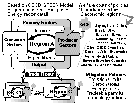
Figure 1. Features of the MIT Emissions Prediction and Policy Analysis
(EPPA) Model.
As summarized in Figure 1, the EPPA model describes the global economy as an interconnected set of national and regional entities, each with supplies of input factors (e.g., labor, capital, land and other resources), consumer demand functions, and production technologies. By providing inputs to the production process, a representative consumer earns the income to purchase final goods, and the circular flow of income and expenditure in such a model is captured in a simplified version of a national accounting system. It is an "equilibrium" model because it finds a set of product and factor prices that balance supplies and demands in each period. It is "general" in that it clears all markets and not just one or two. It is called "computable" because numerical solutions are found with the use of modern digital computers. The EPPA model is "recursive," meaning that it is solved by stepping forward in time, but without the ability to anticipate possible future changes in relative prices, or the imposition of new constraints. It is "dynamic" only in the sense that the capital stocks available in any period are an inheritance from decisions in previous periods.
TABLE 1. Key dimensions of the EPPA model.
Production Sectors
Consumer Sectors
Primary Factors
Regions {and abbreviations}
Gases {and chemical formulae}
Notes:[1] Liquid fuel derived from tars, oil sands, and oil shale, [2] Carbon-free electricity derived from advanced nuclear, solar, or wind, [3] Australia, Canada, New Zealand, EFTA (excluding Switzerland and Iceland), and Turkey, [4] Bulgaria, Czechoslovakia, Hungary, Poland, Romania, and Yugoslavia, [5] OPEC countries as well as other oil-exporting, gas-exporting, and coal-exporting countries. See Burniaux et al., 1992b, [6] Hong Kong, Philippines, Singapore, South Korea, Taiwan, and Thailand
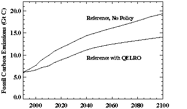
Figure 2. Fossil Carbon Emissions Under the Reference Case, with and without Restriction by a Sample QELRO
Figure 2 shows the global carbon emissions from fossil sources in the Reference case used here. Uncertainties in these predictions are discussed below. Two EPPA predictions are shown, one with no policy and a second which results from our QELRO involving emissions control by OECD nations. As discussed below, the reduction in emissions in the QELRO case is the sum of reductions by the OECD participants in the agreement, and any change in carbon emissions of non-OECD regions because of leakage.The Climate Component of the MIT System | Contents |
When we consider the degree to which the sample policy contributes to larger Convention objectives, we will apply the coupled model of atmospheric chemistry and climate dynamics which also is part of the larger MIT Integrated Global System Model (Prinn et al., 1997). A two dimensional (2D) land- and ocean-resolving statistical-dynamical model is used to address climate dynamics (Sokolov and Stone, 1994). It is a modified version of a model developed at NASA's Goddard Institute for Space Studies (GISS). An important feature of the model, from the point of view of coupling chemistry and climate dynamics, is the radiation code of the GISS general circulation model that it incorporates. This code includes all significant greenhouse gases (H2O, CO2, CH4, N2O, CFCs, etc.), and twelve types of aerosols, whose influence is reflected in the calculations below. Many revisions have been made to the model at MIT, including the incorporation of a real land-ocean distribution, and a capacity to handle alternative formulations of cloud dynamics. In climate simulations, the 2D atmospheric model is coupled to an ocean model with parameterized horizontal and vertical transports.Effects of Emission Restrictions| Contents |
The Distribution of Burdens Among Regions | Contents |
When a carbon constraint is accepted by some regions, the overall system of production, consumption and trade adapts, and the effects are felt both in those countries taking direct action to reduce emissions and in countries that assume no such obligation. The consequences for each region of the sample QELRO, measured in terms of the consumption-based welfare index, are shown in Figure 3. (Note that this welfare measure does not take account of any gains from potential climate effects avoided, or of secondary benefits from the reduction of other pollutants from energy production.) The EPPA model distinguishes four OECD regions: the United States (USA), the European Community (EEC), Japan (JPN) and the Other OECD (OOE). Under the first set of QELRO conditions imposed here, each of these OECD regions meets its emissions target independently (the implications of emissions trading are considered later). The depressing effect on the regional economies of the CO2 constraints, which force adjustments to a lower production frontier and a different composition of output, are clearly shown.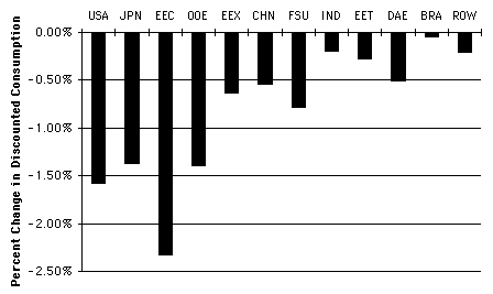
Figure 3. Regional Economic Impacts of Sample QELRO Proposal Computed from Runs of the EPPA Model. Note: Expressed as the cumulative percentage reduction in consumption between 2000 and 2100, discounted at 5%. See Table 1 for regional abbreviations.
Carbon Leakage | Contents |
If one set of world regions constrains activities that produce CO2, then the changes in relative prices and shifts in trade patterns may cause increases in carbon emissions elsewhere, partially offsetting the reductions achieved. This phenomenon is often referred to as the carbon "leakage" which may accompany restrictions that differ among world regions. A number of other studies have considered this phenomenon using multi-region models, including Pezzey (1992), Oliveira-Martins, Burniaux and Martin (1992), Manne and Oliveira-Martins (1994), Edmonds, Wise and Barns (1995), and Golombek, Hagen and Hoel (1995).
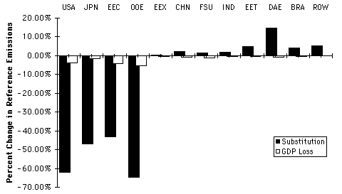
Figure 4. Percentage Change in Carbon Emissions Between 2000 and 2100 due to Substitution Effects and GDP Loss Resulting from a Sample QELRO Proposal. Computed from the differences between two runs of the EPPA model. See Table 1 for regional abbreviations. '
Potential Benefits from Emissions Trading | Contents |
Meeting a commitment to reduce emissions by domestic actions alone is relatively expensive, and countries will seek efficiency by exploiting the cheapest opportunities for reducing carbon emissions, wherever they may be available. One approach is to engage in individual bilateral agreements that allow countries facing a constraint to undertake or fund CO2 reduction measures in other countries. On a project-by-project basis such programs fall under the rubric of Joint Implementation (JI) or Activities Implemented Jointly (AIJ).
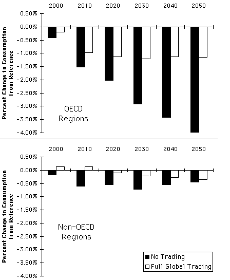
Figure 5. Costs to the OECD of Meeting the Sample QELRO Proposal, with no Emissions Trading and with Global Trading, for Selected Decades. Note: Calculated from runs of the EPPA model.
The Sensitivity of Results to Economic Assumptions | Contents |
Estimates of future greenhouse gas emissions, and of the effects of emission restrictions, are highly sensitive to underlying assumptions about economic conditions over the next century. This fact has been emphasized by a number of studies using emissions models less detailed than EPPA, beginning with early work by Nordhaus and Yohe (1983) and continuing to a number of more recent studies such as those by Dowlatabadi and Morgan (1993) or Hope et al. (1993). Efforts also have been devoted to exploring the uncertainty in multi-region, multi-sector models, examples being those applying the Edmonds-Reilly model (e.g., Edmonds et al., 1986; Margolis; 1995, Tschang and Dowlatabadi, 1995), or Global 2100 (Manne and Richels, 1994 and 1995). To emphasize the importance of this uncertainty for the assessment of proposed QELRO schemes, we have explored the sensitivity of our own model estimates to key inputs. Here we consider three aspects of this issue: overall uncertainty in emissions forecasts, the strong effect of uncertainty about future (backstop) supply technologies, and ways that emissions uncertainty affects one's view of the contribution of proposed control measures to long-run climate goals.Emissions Uncertainty | Contents |
Earlier we identified parameter assumptions that have the greatest influence on future emissions trajectories, including rates of growth of population and labor productivity, the rate of non-price induced improvement in energy efficiency, and the relative costs of the backstop technologies. All these factors are subject to substantial uncertainty. To explore the consequences of this fact, key parameters describing the three most influential of these factors are subjected to an uncertainty analysis, applying a probabilistic collocation method under development at MIT (Webster, Tatang and McRae, 1996; Webster, 1996). The judgment of EPPA model developers was applied to the estimation of probability distributions for these parameters (excluding population growth) [11] and the resulting dispersion of key model outputs was calculated.
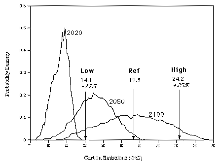
Figure 6. Distribution of CO2 Emissions 2020, 2050, and 2100, Calculated by the EPPA Model. Note: The points R, L, and H indicate 2100 emissions for the Reference, and Higher and Lower scenarios.
Backstop Technologies and Distribution of Burdens | Contents |
Assumptions about the availability and relative cost of the two backstop technologies have an especially significant effect on the distribution of burdens of the QELRO restriction and on estimated leakage. To demonstrate this point, we formulate a case which is dramatically different from that in earlier sections. We hypothesize a world where all the conditions in the Reference case remain the same, except that the backstop technologies do not exist (or, alternatively, that their costs are so high that they never enter substantial use). The stark comparison is particularly useful in illuminating the mechanisms that distribute the economic burden among regions. The carbon-free and carbon fluids backstops partially counteract one another. Thus the Reference case with no backstops implies total carbon emissions that total about 14% more than the Reference with both backstops (with no emissions limits in either case). The no-policy pattern of regional emissions is even more significantly different between the two worlds, owing to differences in penetration of the two backstops, as are the levels of GDP and of our consumption-based welfare measure.
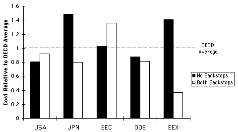
Figure 7. Costs of the Sample QELRO, for the Reference Case with and without Backstop Energy Sources, Stated as a Multiple of the OECD Average Cost in Each Case.
For example, Europe, was relatively disadvantaged in a world with backstops (see Figure 7 and Figure 3) because it lacks the resources to support the carbon intensive backstop, and the carbon-free electric backstop is expensive relative to conventional costs. If no region has these technologies, then the cost to Europe is near the OECD average. Japan, on the other hand, is a relative loser among OECD countries in a world without backstops. Recall that one factor that made the QELRO relatively easy to meet in a world with backstops (see Figure 3) was the fact that the cost of the carbon-free backstop in Japan was not far above its 1990 conventional power costs, so the transition to this technology helped meet the QELRO at a relatively low burden. Without it, Japan is substantially disadvantaged. The United States and the Other OECD (OOE) are similar to one another in economic structure in a world with backstops (both have the carbon-fuels technology), and in a world without them as well, and their QELRO costs are somewhat below the OECD average in both cases. Contribution to Goals of the Climate Convention | Contents |
Finally, there is the issue of the significance of this sample QELRO in advancing the stabilization goal laid out in the Framework Convention on Climate Change. The answer to this question can be seen in the effects of such an agreement on the trajectories of atmospheric CO2 concentrations, and of global mean temperature. Shown in Figure 8 and 9 are results from the MIT Integrated Global System Model, for the Reference case used above and for alternative predictions chosen from the distribution in Figure 6 (where they are indicated as High and Low). The High and Low cases are set to be 1.5 S.D. above and below the mean (which is very close to the Reference case) of the distribution of total carbon emissions over the century. [13] Among the many parameter combinations that will yield cumulative emissions at these two levels, the ones with the highest joint probability of occurrence were selected. A "reference" version of the coupled chemistry-climate model (Prinn et al., 1997) is used in all cases. [14]
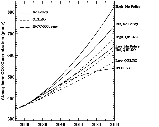
Figure 8. Forecasts of CO2 Concentrations for Reference, High and Low Emissions Cases, with and without QELRO Restriction. Note: An IPCC concentration path for a 550 ppmv goal also is shown.
Figure 8 shows the paths of CO2 concentrations in parts per million by volume (ppmv) in air, with and without the QELRO agreement, for the Reference (Ref) and High and Low cases. In the absence of policy of restriction, the Reference prediction is 742 ppmv by 2100. The range of economic predictions leads to CO2 levels between 645 ppmv and 834 ppmv (from 12% below to 14% above the Reference case, or a 26% range). The effect of the restriction adopted by the OECD is to lower the predicted 2100 concentrations. For example, under the Reference conditions the sample QELRO lowers the 2100 concentration from 742 ppmv to 629 ppmv (16%). Naturally, because the QELRO holds OECD emissions to the same fixed level in all cases, the policy effect is greater in the High emissions case (lowering from 834 ppmv to 688 ppmv or 18%), and smaller under the Low case (dropping from 645 ppmv to 574 ppmv or 11%). Interestingly, the effect of the sample QELRO on CO2 concentrations in 2100 is less significant than the emissions uncertainty alone, as tested in these experiments.
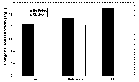
Figure 9.Change in Global Mean Temperature from 1977 to the 2090-2100 Decadal Average, for Reference, High and Low Emissions Cases, with and without QELRO Restrictions
Concluding Observations | Contents |
References | Contents |
Armington, P.S. (1969). "A Theory of Demand for Products Distinguished
by Place of Production," Int. Monetary Fund Staff Papers, 159-176.
Burniaux, J., G. Nicoletti and J. Oliveira-Martins (1992a). GREEN: A Global Model for Quantifying the Cost of Policies to Curb CO2 Emissions, OECD Economic Studies No. 19, Paris.
Burniaux, J., J.P. Martin, G. Nicoletti and J. Oliveira-Martins (1992b). GREEN - A Multi-Sector, Multi-Region General Equilibrium Model for Quantifying the Costs of Curbing CO2 Emissions: A Technical Manual, OECD Economics Department Working Paper No. 116, Paris.
Dowlatabadi, H. and M.G. Morgan (1993). "A Model Framework for Integrated Studies of the Climate Problem," Energy Policy 21 (3), 209-221.
Edmonds, J. and D.W. Barns (1992). "Factors Affecting the Long-Term Cost of Global Fossil Fuel CO2 Emissions Reductions," International Journal of Global Energy Issues 4(3), 140-166.
Edmonds, J.A., J.A. Reilly, J.M. Gardner and A. Brenkert (1986). "Uncertainty in Future Energy Use and Fossil Fuel CO2 Emissions 1975 to 2025," Report No. DOE/NBB-0081, Office of Energy Research, U.S. Department of Energy, Washington, D.C.
Edmonds, J., M. Wise and D.W. Barns (1995). "Carbon Coalitions: The Cost and Effectiveness of Energy Agreements to Alter Trajectories of Atmospheric Carbon Dioxide Emissions," Energy Policy, 23(4/5), 309-335.
Golombek, R., C. Hagen and M. Hoel (1995). "Efficient Incomplete International Climate Agreements," Resource and Energy Economics 17 (1), 25-46.
Hope, C.H., J. Anderson and P. Wenman (1993). "Policy Analysis of the Greenhouse Effect: An Application of the PAGE Model," Energy Policy 21 (3), 327-338.
IPCC (1995). Climate Change 1994 - Radiative Forcing of Climate Change and an Evaluation of the IPCC IS92 Emissions Scenarios, Contribution of Working Group I of the Intergovernmental Panel on Climate Change, Cambridge University Press, Cambridge, UK.
IPCC (1996a). Climate Change 1995 - The Science of Climate Change, Contribution of Working Group I to the Second Assessment Report of the Intergovernmental Panel on Climate Change, Cambridge University Press, Cambridge, UK.
IPCC (1996b). Climate Change 1995 - Economic and Social Dimensions of Climate Change. Contribution of Working Group III to the Second Assessment Report of the Intergovernmental Panel on Climate Change, Cambridge University Press, Cambridge, UK.
Jacoby, H.D. and R. Prinn (1994). Uncertainty in Climate Change Policy Analysis, MIT Joint Program on the Science and Policy of Global Change, Report No. 1, Cambridge, MA.
Manne, A.S., and J. Oliveira-Martins (1994). "Comparison of Model Structure and Policy Scenarios: GREEN and 12RT," OECD Economics Department Working Paper No. 146, Paris.
Manne, A.S., and R.G. Richels (1994). "The Costs of Stabilizing Global CO2 Emissions: A Probabilistic Analysis Based on Expert Judgments," The Energy Journal 15(1), 31-56.
Manne, A.S. and R.G. Richels (1995). "The Greenhouse Debate: Economic Efficiency, Burden Sharing and Hedging Strategies," The Energy Journal, 16(4), 1-37.
Margolis, R.M. (1995). "Probabilistic Policy Experiments: The Use of Energy-Economic-Environmental Models in the Climate Change Policy Process," International Journal of Environment and Pollution 5(1), 1-20.
Martin, J.P., J. Burniaux, G. Nicoletti and J. Oliveira-Martins (1992). "The Costs of International Agreements to Reduce CO2 Emissions: Evidence from Green," OECD Economic Studies 19, Paris, 93-121.
Nordhaus, W.D. and G.W. Yohe (1983). "Future Carbon Dioxide Emissions from Fossil Fuels," Climate Change: Report of the Carbon Dioxide Assessment Committee, National Academy of Sciences, Washington, D.C.
Oliveira-Martins, J., J-M. Burniaux, and J.P. Martin (1992). "Trade and the Effectiveness of Unilateral CO2-Abatement Policies: Evidence from GREEN," OECD Economic Studies 19, Paris, 123-140.
Pezzey, J. (1992). "Analysis of Unilateral CO2 Control in the European Community and OECD," The Energy Journal 13(3), 159-171.
Prinn, R., et. al. (1997). "Integrated Global System Model for Climate Policy Analysis: Feedbacks and Sensitivity Studies," submitted to Climatic Change, March 1997.
Sokolov, A.P. and P.H. Stone (1995). Description and Validation of the MIT Version of the GISS 2D Model, MIT Joint Program on the Science and Policy of Global Change, Report. No. 2, Cambridge, MA.
Tietenberg, T., and D. Victor (1994). "Administrative Structures and Procedures for Implementing a Tradeable Entitlement Approach to Controlled Global Warming," in Possible Rules, Regulations and Administrative Arrangements for a Global Market in CO2 Emission Entitlements, UNCTAD/GID/8, Part I.
Tschang, F.T. and H. Dowlatabadi (1995). "A Bayesian Technique for Refining the Uncertainty in Global Energy Model Forecasts," International Journal of Forecasting 11 (1), 43-61.
United Nations (1992). "Framework Convention on Climate Change," International Legal Materials 31, 849-873.
United Nations (1995). "Report of the Conference of the Parties On Its First Session, Held at Berlin from 28 March to 7 April 1995," Framework Convention on Climate Change, Conference of the Parties, FCCC/CP/1995/Add 1, 6 June.
United Nations (1997). "Framework Compilation of Proposals from Parties for the Elements of a Protocol or Another Legal Agreement," Framework Convention on Climate Change, Ad Hoc Group on the Berlin Mandate, FCCC/AGBM/1997/2, 31 January.
Webster, M.D., M.A. Tatang, and G.J. McRae (1996). Application of the Probabilistic Collocation Method for an Uncertainty Analysis of a Simple Ocean Model, MIT Joint Program on the Science and Policy of Global Change, Report No. 4, Cambridge, MA.
Webster, M.D. (1996). Analysis of Uncertainty in Large Models with Application to Climate Policy, MS Thesis, Massachusetts Institute of Technology, May.
Wigley, T., R. Richels and J. Edmonds (1996). "Economic and Environmental Choices in the Stabilization of Atmospheric CO2 Concentrations," Nature 379, 18 January, 240-243.
Yang, Z. et al. (1996). The MIT Emissions Prediction and Policy Assessment (EPPA) Model, MIT Joint Program on the Science and Policy of Global Change, Report No. 6, MIT, Cambridge, MA.

--> Home Page | Report Series | Table of Contents |