Instructor
Anastasia Yendiki, Ph.D.
Lab description
The purpose of this lab is to familiarize you with the
preprocessing steps performed on fMR images prior to linear modeling
and with the issues and limitations of fitting a linear model to
data from a single functional run.
Lab software
We will use NeuroLens
for all fMRI statistical analysis labs.
Lab data
We will use data from the self-reference functional paradigm
that was presented in Lab 1. For this lab we will only use data
from Subject 7, available under the course directory:
/afs/athena.mit.edu/course/other/hst.583/Data2006/selfRefOld/Subject7Sessions7-8-9-13/
Here's a reminder of the paradigm structure.
Words are presented in a blocked design.
Each run consists of 4 blocks,
2 with the self-reference condition and
2 with the semantic condition.
The conditions alternate in the ABBA format.
In particular, for Subject 7 the order is:
Run 1:  A=semantic, B=selfref
Run 2:  A=selfref,  B=semantic
Run 3:  A=semantic, B=selfref
Run 4:  A=semantic, B=selfref
Words are presented for 3 sec each, grouped in blocks of ten. Prior to each block the subject views a 2 sec cue describing their task for the upcoming block. Each block is followed by 10 sec of a rest condition. This is the breakdown of a single run:
10 sec   Rest
2 sec    Cue
30 sec   Block A (10 words, each lasts 3 sec)
10 sec   Rest
2 sec    Cue
30 sec   Block B (10 words, each lasts 3 sec)
10 sec   Rest
2 sec    Cue
30 sec   Block B (10 words, each lasts 3 sec)
10 sec   Rest
2 sec    Cue
30 sec   Block A (10 words, each lasts 3 sec)
16 sec   Rest
----------------------------------------
TR = 2 sec
Total run duration = 184 sec (i.e., 92 scans) per run
Lab report
The lab report must include your answers to the questions found
throughout the instructions below.
Due date: 11/20/2006
-
We will begin by setting up a design matrix for
the general linear model, based on the
paradigm description above.
We will save the design matrix in a text file,
so that we can load it into NeuroLens whenever
we want to analyze data from the self-reference paradigm
in this and subsequent labs.
Open a new text file using TextEdit
(the text editor found in the Applications folder of your Mac)
or any other text editor.
Enter first the design matrix column corresponding to the self-reference condition in the first run. It must contain 92 digits (one for each TR). Each digit must be 1 if the self-reference condition is on during that TR, or 0 otherwise. Then enter the design matrix column corresponding to the semantic condition in the first run (another set of 92 digits).
White space is ignored by NeuroLens, but you can use it to make your file readable and easier to check. When you are done, save the file with a name like selfref,runs1,3,4.txt to indicate that it reflects the timing of runs 1, 3 and 4. (Run 2 will need a different design matrix.)
-
Open the Subject 7 data by dragging its entire folder
onto the NeuroLens icon (or by starting NeuroLens
and choosing Open... from the File menu).
Then double-click on the first run in the list of data sets
(Series 7):
-
We will first try analyzing the data from this run without
any preprocessing. From the Action toolbar item,
choose Linear Modeling.
In the Design tab, press the Read file... button and choose the text file you created in Step 1. Fill in the TR in the Time step field.
In the Contrasts tab, set up 3 contrasts:
- Self-reference condition vs. baseline
- Semantic condition vs. baseline
- Self-reference condition vs. semantic condition
In the HRF tab, keep the default parameters for the HRF shape.
In the Model tab, choose 1 (Linear) from the Polynomial drift order menu.
In the Output tab, check T-statistic, -log(p), and Signal-to-noise ratio.
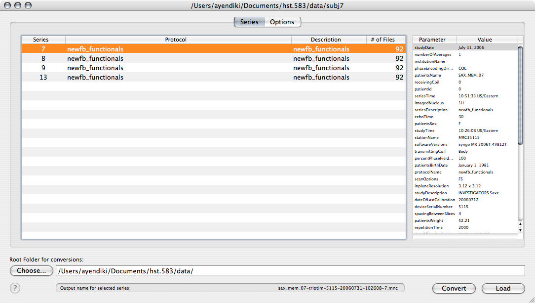
When you are done setting up the model, click on the Run button to fit the linear model. The first 3 new windows that you get should show the T-map volumes corresponding to the 3 contrasts:
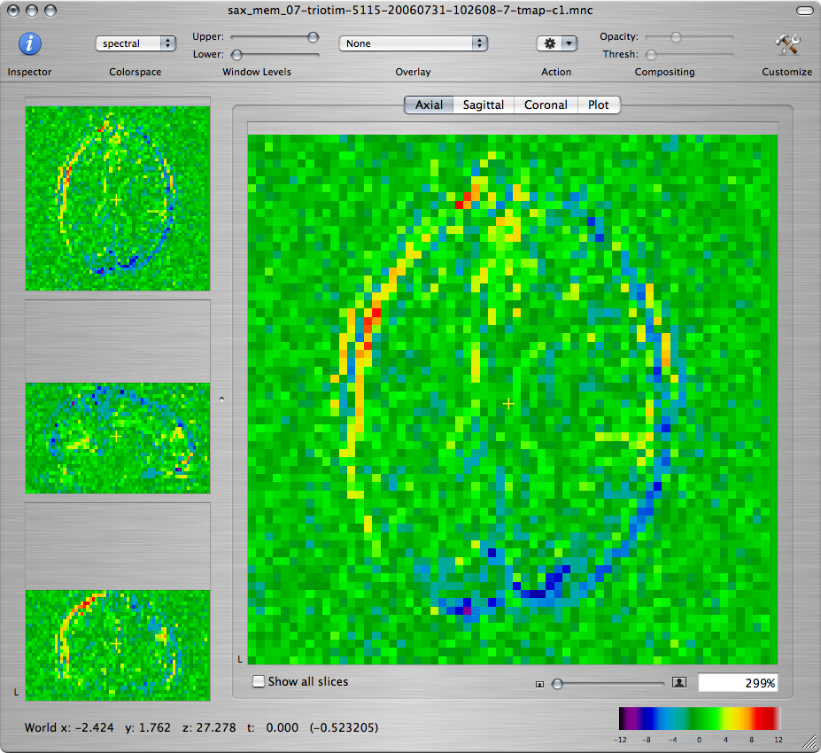
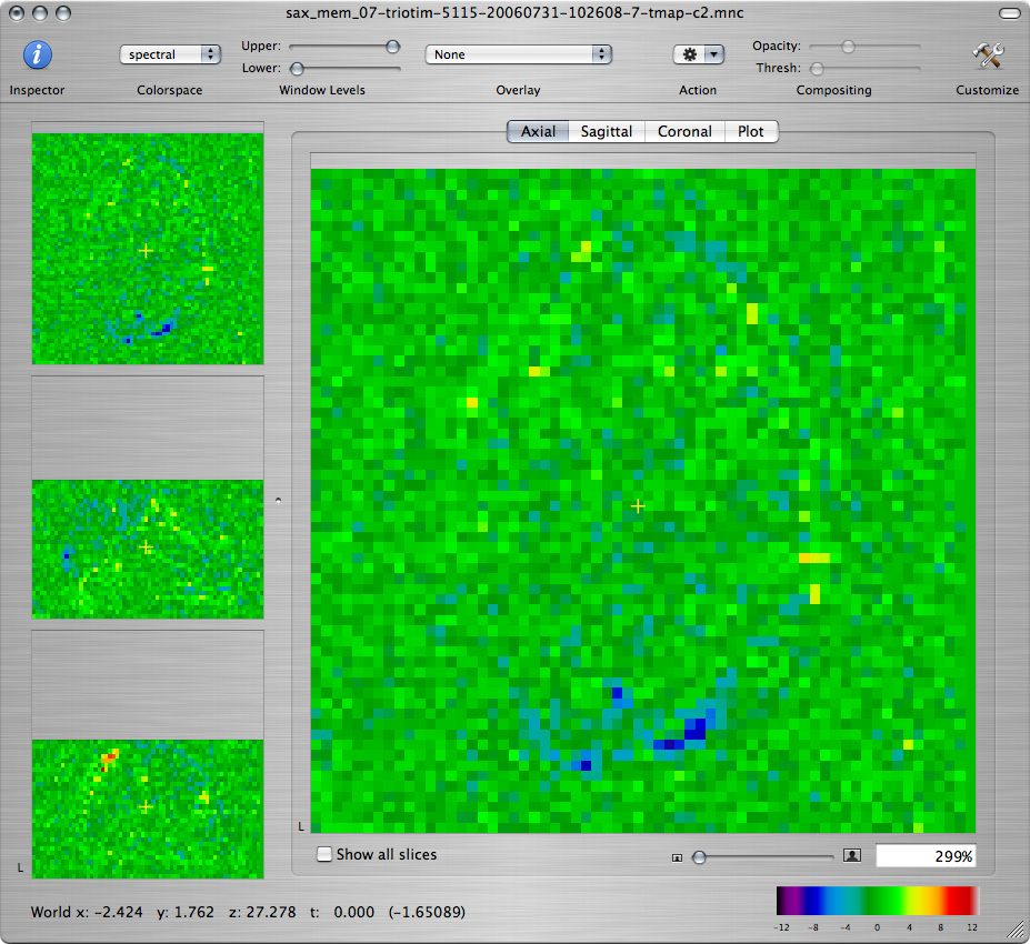
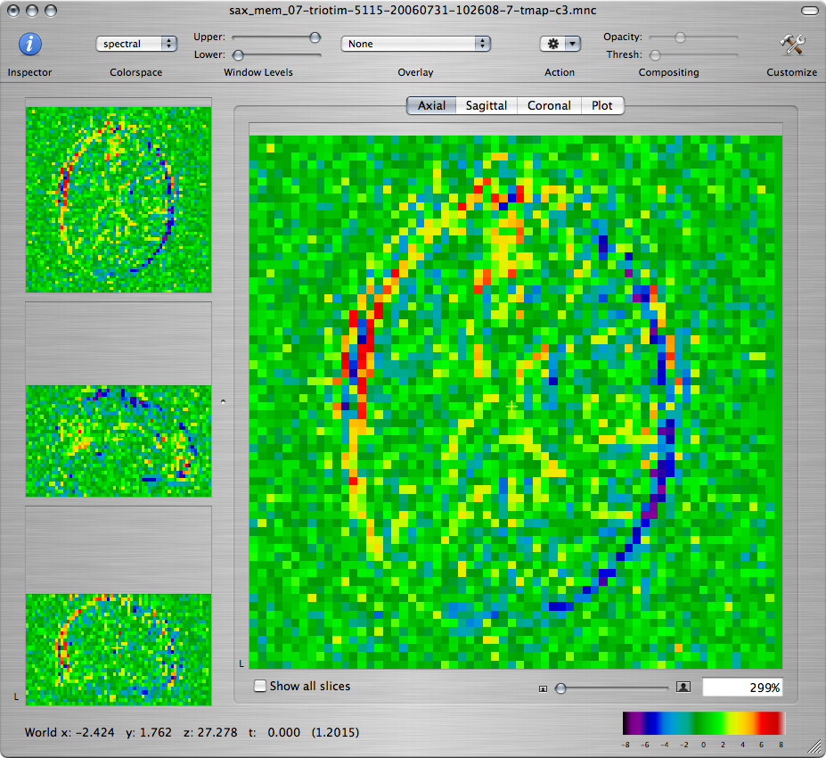
Q: Scroll through the maps and describe what you see. Is this a good fit to the functional paradigm? Explain the activation that you observe and the differences between the T-maps corresponding to the three contrasts.
If you think you may want to return to these T-maps when you are writing up your report, you can save them as .mnc files by selecting the window of each map and choosing Save As... from the File menu. You can now close all the windows that have been output by the linear modeling.
-
Next we will apply motion correction to the images and reanalyze them.
Go to the window showing the original functional images.
From the Action toolbar item, choose Motion Correction.
In the Basic tab, enter the number of the middle time frame in the Target Frame field.
In the Outputs tab, check Motion parameters.
Click the OK button to run the motion correction. You should get 3 new windows. One of the windows shows the motion-corrected images and the other two show plots of the estimated motion parameters:
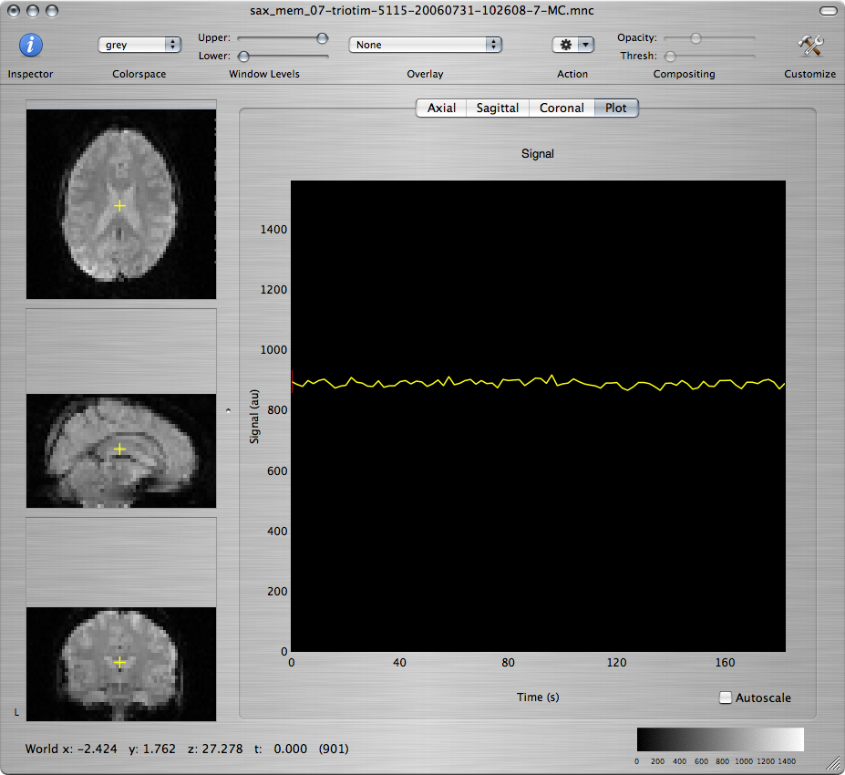
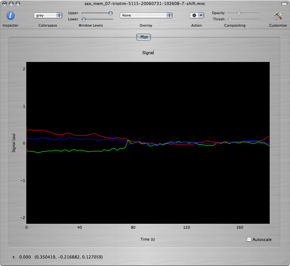
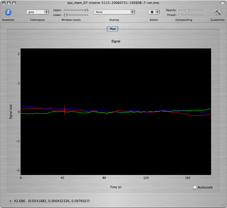
Q: Based on the estimated motion parameters, what are the main types of motion that have been detected in this data set? What was happening in the experimental paradigm when the most severe motion occured?
-
Rerun the linear model fitting from Step 3, this time
on the motion-corrected data set.
Scroll through the T-map for Contrast 1 to scan for brain regions with large positive values. Command-click on several voxels within those regions to inspect the model fit of the timecourse at those voxels, as seen in the window showing the motion-corrected data set.
Q: Report the approximate coordinates of the center of each region that shows robust activation and good fit to the model. What are the functions that these regions support based on the subject's neuroanatomy? How are your findings explained by what is going on in the experimental paradigm?
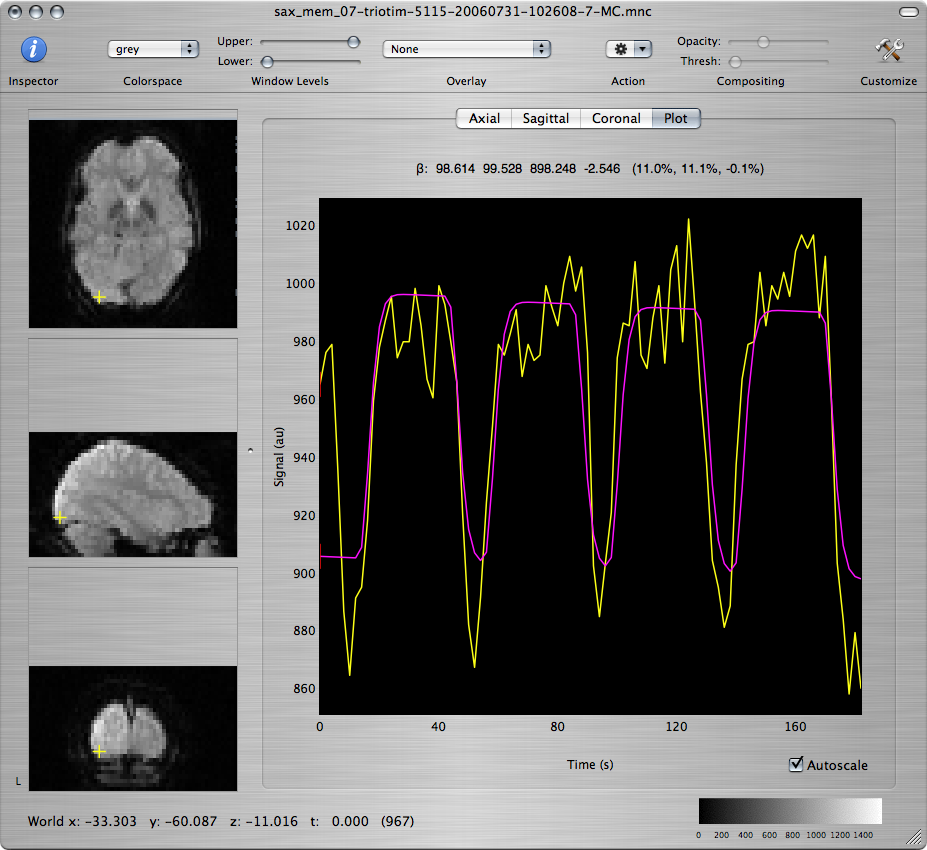
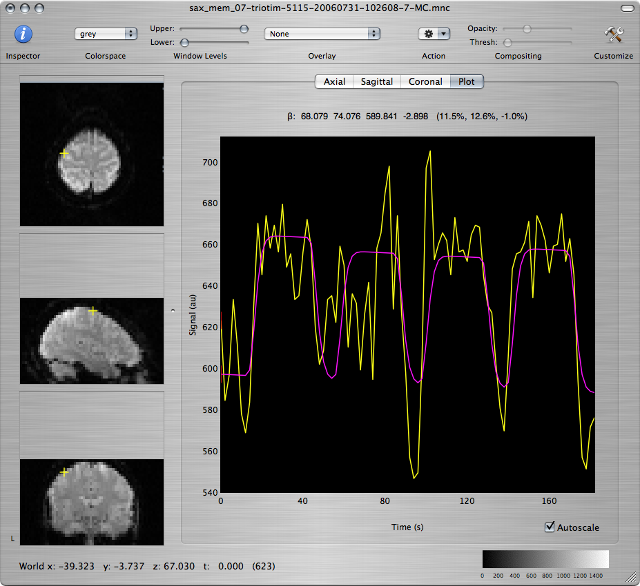
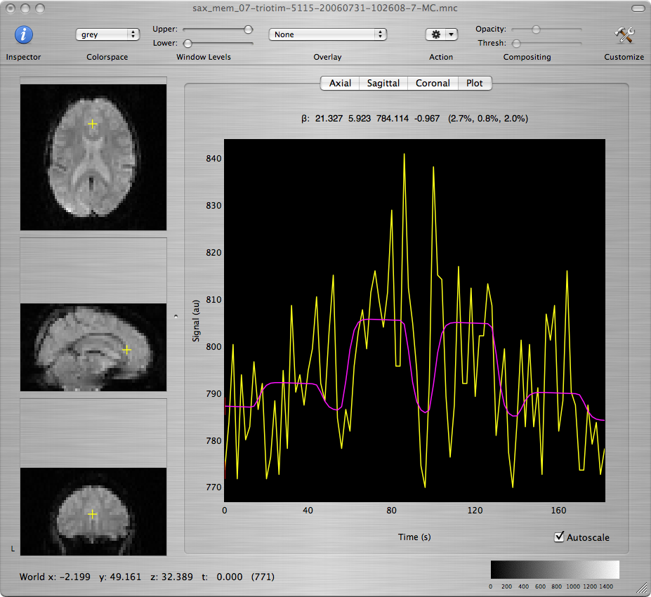
Q: Repeat for the T-maps corresponding to Contrasts 2 and 3 and discuss differences and similarities among the 3 maps.
-
We will now draw a region of interest (ROI)
that we will use to investigate the effects of spatial smoothing.
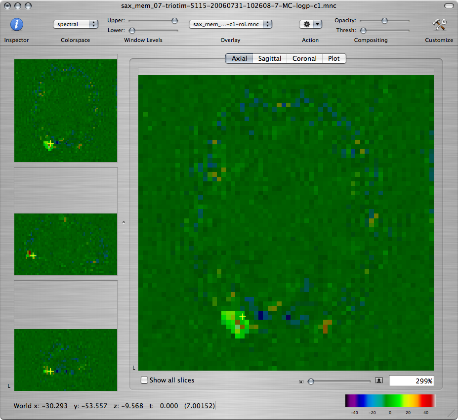
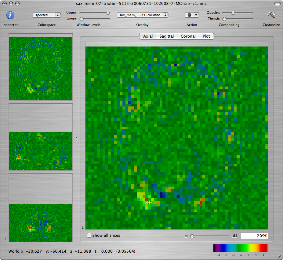
Scroll through the axial view of the -log(p) map for Contrast 1
and find the axial slice with the greatest activation
in the visual area. We will draw a ROI around that activation.
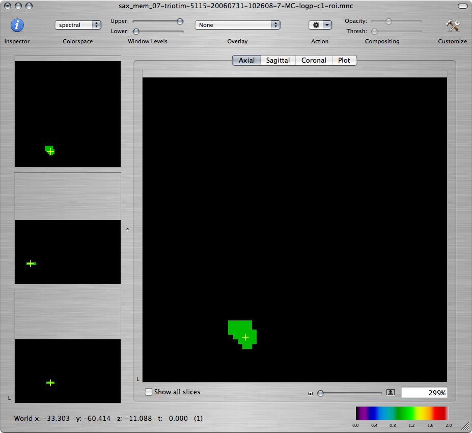
Create a new overlay by choosing Create Overlay from the File menu. (You must make sure to draw the ROI on the overlay. Drawing directly on one of the maps will change the map values.) While pressing Shift, draw the outline of the ROI so that it encompasses a generous area around the high activation.
To make the ROI more visible, you can increase its opacity by clicking on the Inspector toolbar item and using the Opacity slider in the Image tab.
The ROI should appear both in the window of the -log(p) map as an overlay, and in its own window that's named *-roi.mnc. (You may have to Command-click inside the ROI in the -log(p) window to make the right slice appear in the ROI window.)
-
We are now ready to record a set of measures for this ROI,
which we will repeat with different levels of smoothing.
For your convenience, you can use the table at the bottom
of this page to write down the values.
To view ROI statistics, click on the Inspector toolbar item. In the Inspector window, click on the ROI tab and check Compute ROI statistics:
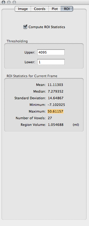
Q: Record the maximum value of -log(p) within the ROI.
Go to the window showing the SNR map for Contrast 1. From the Overlay toolbar item, choose the ROI of the visual area that you drew. As above, open the Inspector window and compute the ROI statistics:
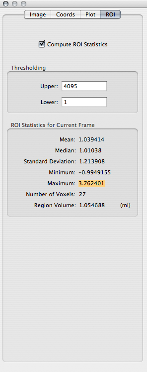
Q: Record the maximum value of SNR within the ROI.
-
We will now explore the effects of smoothing the images
prior to statistical analysis.
Go to the window showing the
motion-corrected functional images. From the Action toolbar item, choose Spatial Smoothing.Select a Gaussian smoothing kernel. Enter 3 in the Width field AND THEN PRESS TAB - NeuroLens will not read the new width value unless you press tab! %-( Click on the OK button to smooth the motion-corrected images with the selected kernel.
Rerun the linear model fitting from Step 3, this time on the smoothed, motion-corrected data set. Repeat step 7 to compute the ROI statistics on the smoothed results.
Repeat these steps, changing the FWHM of the Gaussian smoothing kernel to 6, 9 and 12 mm. (Each time apply the spatial smoothing to the unsmoothed motion-corrected data set, not to a previously smoothed data set.)
Q: Use a program of your choice (Matlab, Excel, etc.) to make plots of the maximum SNR and maximum -log(p) within the ROI as a function of smoothing FWHM (from 0 to 12 mm). Show your plots with labeled axes.
-
Repeat the above measurements for the ROI
of a cerebellar activation that you can find under:
/afs/athena.mit.edu/course/other/hst.583/Data2006/selfRefOld/subj7,run1,roi,cerebel.mnc
Q: Plot the maximum SNR and maximum -log(p) within the cerebellar ROI as a function of smoothing FWHM (from 0 to 12 mm). How are the benefits of spatial smoothing different or similar in the visual and cerebellar ROIs? Is there a universally optimal width for the smoothing kernel? How do you explain this result?
-
Q: Has spatial smoothing altered your conclusions about robustly activated regions from Step 5? Have the self-reference-vs.-semantic activation clusters that you expect from the discussion of Lab 1 shown up in a statistically significant way? Why (not)?
Smoothing FWHM (mm) Max -log(p) visual Max SNR visual Max -log(p) cerebellar Max SNR cerebellar 0 3 6 9 12