2D Polygon Morphing
using the
Extended Gaussian Image
Manolis Kamvysselis
|
1. Introduction
|
2. Algorithm
|
3. Implementation
|
4. Results
|
|
1. Introduction
|
2. Algorithm
|
3. Implementation
|
4. Results
|
Morphing techniques that have been developed to progressively transform one two-dimensional image to another are usually pixel based and morph a source to a target by interpolating pixel values based on constraints specified by the user.
In this work, we are using a model-based approach to propose a solution to morphing a two-dimensional polygon into another. Our model of an object will be its Extended Circular Image representation, the two-dimensional equivalent of the Extended Gaussian Image. This approach will work only for convex polygons, for which the ECI is unique.
To morph non-convex polygons, one would have to separate them into convex components and morph each separately, or use an extended version of the ECI that would apply to non-convex polygons. This morphing method can be applied to convex polyhedra using the Extended Gaussian Image, and similarly be extended to non-convex polyhedra.
This term, I was working on a model-based three-dimensional morphing project for Computer Graphics.
The algorithm I developed for that project was simply matching polygons in a three-dimensional world in a nearest-neighbor fashion, and growing unmatched polygons from zero-area polygons on edges of other polygons.
The results of this approach were often quite satisfactory both graphically and mathematically, the polygons indeed traveling the way I hoped they would. However, the algorithm never assumed that the source or target objects were connected, and sometimes broke the connectivity which should have been preserved.
Having explored the unconnected case, I decided to explore the other extremity, where we assume that all polygons are connected. Including the additional constraint that those closed objects are convex, we can use the Extended Gaussian Image representation of an object to uniquely define it in 3D.
The problem therefore becomes that of moving the weights of the EGI on the unit sphere to redistribute them such that the EGI of the source polyhedron becomes that of the target, while keeping the center of mass at the origin (so that all intermediate objects are closed themselves).
This approach allows us to get around the problem of matching two objects of different connectivity by letting the inverse EGI function create faces of arbitrary shape, our program having specified only their size and normal direction by moving the weights on the three dimensional sphere.
The current algorithms for computing the inverse EGI being
incremental, we are optimistic about this approach since the
difference in connectivity and shape between two morphing steps will
generally be small, allowing a faster computation of the inverse EGI.
The current two-dimensional algorithm is
Many approaches are possible for transforming the source normals
to the target normals. Each corresponds to a different way of
picturing the problem to solve. All approaches must make sure that the
weights have their center of mass at the center of the unit circle at
every intermediate step, such that convexity is preserved.
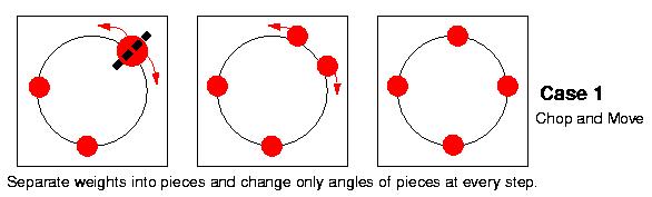
One could picture the normals as physical weights on a sphere and thus want to simply interpolate angles of the normals, unable to take weight from one normal to another across the sphere. This approach will break each source weight into many chunks and it will then move those pieces of constant weight around the sphere until they recombine into the target ECI.
Alternatively, one could consider the angles of the normals as the only places on the sphere where a weight could appear, as liquid containers all connected to each other, the weight being the quantity of liquid that we would pour into each container. We'll then simply transfer weights between normals at every step.
We'll describe the general case as a combination of those two basic movements described above. Every normal will be allowed to move on the sphere, while distributing its weight to other normals and collecting weight from them. One can integrate both movements by matching initial and final angle and weight for every normal increment, and linearly interpolating both angle and weight. One has to then prove that the center of mass of the increments is the center of the ECI circle, to guarantee that every intermediate step will be a closed polygon.
Except from how much the angles will change and how much the weights will change, one has to make more decisions, such as which normals are affected by which others. Many choices are possible, ranging from the case where every normal is affected by and affects only the normals closest on its right and left (could be only two, or all those needed to sum up the normal's weight), to the case where every normal affects and is affected by all the other normals.
Those decisions will lead to intermediate objects with different
characteristics. Intermediate edges can be small, yielding smooth
objects, circular at the extreme case, or they can be larger,
minimizing creation and deletion of faces, and thus conserving the
topological similarities between source and target as much as
possible. The right balance between smooth transitions and topology
preservation is often an aesthetic decision of the user, and neither
approach can be argued more correct than the other.
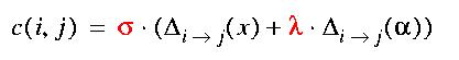
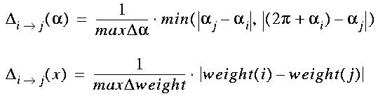
In our approach, each normal is compared with all other normals,
and a cost c(i,j) of transforming every source to every target is
calculated as follows:
where Delta(a) is the minimum angle difference between two normals
(cycling around 2*pi if necessary), and Delta(w) is the weight
difference between the normals. Both deltas are scaled to fit a
[0..1] range, such that matching is independent of the coordinate
system.
Moreover, we use a lambda factor to multiply one of the two
differences (here, the angle), such that a change in angle costs more
than an equivalent change in weight, so that we can emphasize the
properties we'd like to see preserved in our morphing.
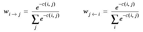
Those costs are then entered into a function that guarantees that
the center of mass of the ECI is preserved throughout the morphing
process, and that intermediate polygons will also be closed. I owe
this function to Panayiotis (Peter) Kamvysselis (pkamvyss@mit.edu), my
older brother, with whom I discussed this interesting problem of
matching normals on a unit sphere for morphing, and whose ideas and
opinions were very helpful. We calculate the source normal portion
corresponding to the part of the i-th normal that goes to the j-th
source, by scaling the i-th normal by w(i->j) below, and the target
normal portion received by the jth target from the ith source is
obtained by scaling the jth target by w(j<-i) below. The function used
is:
This function allows for each normal to be morphed into only one
other normal, if the match is very good, or contribute slightly to all
other normals, if no good match exists. The appearance of the
intermediate objects therefore depends on the quality of the existing
matches, according to the criteria specified by the lambda above, but
also on the variance 1/sigma of the function, which appears as a
scale factor of the total cost c(i,j).
As a proof of concept, you can find a two-dimensional version of
the algorithm at MMorph.html.
The Java byte code is available at MM*.class, and the source is at MM*.java.
The following links will lead you to the source code of individual files of the code of the program. Feel free to use part or all of it, while giving credit to the author (Manolis Kamvysselis -- manoli@mit.edu -- http://web.mit.edu/manoli/www/).
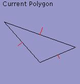
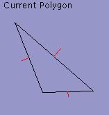
When lambda (which multiplies the angle change) is small (less
than 1), what really matters in our cost function is the change in
weights, by the formula above. The program will
therefore break the edges into components which don't have to be
scaled, but simply rotated, such as to minimize scaling cost.
Since the angle of the edge components will be interpolated linearly,
from their source orientation to their destination orientation, the
external angles shown in the diagram above will be minimized, yielding
smoother intermediate polygons, with smoother angle transitions.
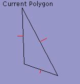
The same source and target triangles presented in the two previous
examples can also be transformed into one another by a simply rotation,
which the program has found by increasing the angle cost a little more.
This transformation, obviously minimizing weight change, apparently also
minimizes rotation angle, since only three sides are rotated.
The results of this project leave us optimistic about the
three-dimensional case, at least for the normal matching on the unit
sphere. The recovery of the polyhedron from the interpolated Gaussian
Image is still generally little known and expensive, but we have
interesting ideas for improving the reverse EGI operation based on the
tons of information provided by known polyhedral models of neighboring
EGIs.
Matching Weights
Implementation
Program
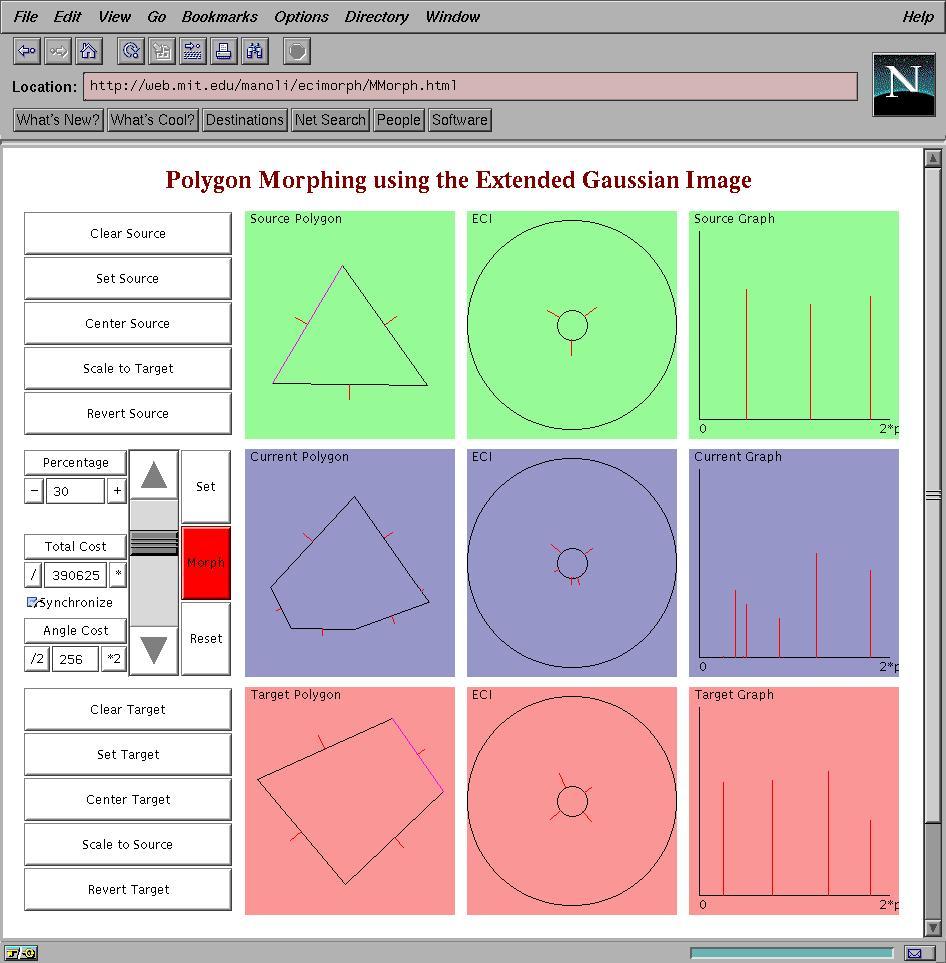
Using the program
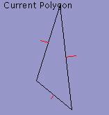
To morph two polygons
Parameters
Buttons
Code
Results
Types of morphing
Smoothest
Balanced
Rotation
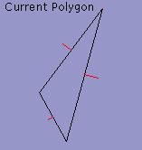
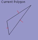
Source
20%
40%
60%
80%
Target
Smooth
Balanced
When lambda is larger, the intermediate polygons tend to have larger
edges. The program will match source normals to target normals with
nearby angles, even if the weights have to be scaled, since the cost
of scaling decreases as the cost of rotating increases. The second
column above shows a balance between rotation and scaling obtained
with lambda = 1.
Rotation
More
Feel free to play around with more examples.
Future Work
Prof. Berthold K P Horn - Manolis Kamvysselis - manoli@mit.edu - December 20, 1997