3D Morphing
Manolis Kamvysselis - Matt D. Blum - Hooman Vassef - Krzysztof Gajos{ manoli - mdblum - hvassef - kgajos } @mit.edu
Pipeline
Ideas
Rendering
Algorithm
Future
Examples
Slides


|
|
3D MorphingManolis Kamvysselis - Matt D. Blum - Hooman Vassef - Krzysztof Gajos{ manoli - mdblum - hvassef - kgajos } @mit.edu | |
|
Jump to: Pipeline Ideas Rendering Algorithm Future Examples Slides |
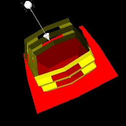
Click on the icons below to see morphing animations
| |
This paper presents our work towards achieving a model based approach to three dimensional morphing. It describes the initial algorithms and ideas that we envisioned, the final algorithm we developed and implemented, the environment we worked in, our visualization techniques, and future work planned on the subject.
A better way to accomplish two-dimensional morphing is to identify line segments on the source image with line segments on the target image so that pixel values will actually move across the image so that features will be preserved better. For example to map a face to another face, it is important that certain features such as the eyes, nose, and mouth are identified so that intermediate images actually look natural. The mouth of the source image will move to the proper place in the target image.

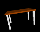
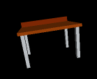
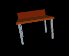
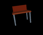
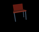
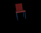
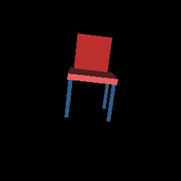
The three-dimensional morpher creates intermediate scenes, calculating the geometry of every scene that falls between the source and the target. In Figure 2 (obtained using our program), every intermediate object between a table and a chair, is an object by itself, and it's hard to know when the object stops being a table and starts being showing smooth transitions of geometry as well as the color varying continuously.
It is easy to describe the basic algorithm in words, but such a mapping scheme of triangles is harder than one would initially think. What happens for example if the two scenes contain different numbers of triangles or the triangles are connected in different ways in the two scenes? That is, how do we handle topologically different objects?
Our primary goal was to create a program by which we could morph two polyhedral objects into one another. for the morphing algorithms, we considered several approaches before implementing the final algorithm.
Using the SGI's as a platform, we decided to take to our advantage the Open Inventor library, including the triangulation routine used in the ivscan program. Our program takes as an input a number of frames k and two Inventor files, preferably written following some basic rules. It feeds them trough a pipeline, and displays the k intermediary objects that it created using the morphing algorithm between the source and target objects. Also, using an off-screen renderer, we can create a sequence of *.gif files (see Figure 2).
It has to be mentioned at this point, that certain components of our program are adaptations of the IvScan code.
Below there is a schematic diagram representing the architecture of our program. A more detailed explanation of each component follows.
![The schematic
diagram of the structure of our program
[Click to Enlarge]](graphics/pipeline.gif)
1. Read .iv files Reads the source and target files in Inventor format. Builds source and target Inventor objects.
2. Split Removes the
top level Separators in both objects. Assumes that all children of the
top Separators are also of type SoSeparator. It matches the first
child of the source with the first child of the target, etc. If
numbers of children in the two objects are not equal, the matching is
done for the smaller number of children. The pairs of source-target
subobjects will be put through the rest of the pipeline separatelly
until they are to be displayed. At that point, a top level Separator
will be added to gather them all.
The motivation for incuding
splittin in the pipeline was to allow users to specify somehow which
parts of one object should be morphed into what parts of the target
object.
The reason why we do it in the manner described above is
because we were looking for a method that would be both easy to use
and easy to implement.
Note: Because of how we split objects into subobjects, all the second level nodes in the input objects HAVE TO BE OF TYPE SoSEPARATOR.
3. Triangulize Use the Triangle CallBack supplied by Inventor to split the subobjects into triangles. At that point, we store the objects in our own datastructure.
4. Scale & Translate
Find the extreme points of each subobject. Then scale and translate it
so that it first inside a unit cube. This little bit of pre-processing
makes the design and implementation of the morphing algorithm
significantly easier.
Information on how much the object was
scaled and translated is saved so that later on the object can be
restored to its original position and size.
5. ![]() At this point the
pipeline is stopped until all the subobjects complete the previous
steps. As soon as all of them are done we go to the next step, which
is...
At this point the
pipeline is stopped until all the subobjects complete the previous
steps. As soon as all of them are done we go to the next step, which
is...
6. Morphing! Yes, this
is where an intermediate object is created. The intermediate object is
created of a set of triangles. The vertices of these triangles contain
their source and target coordinates as well as the coordinates of the
current position and other information needed while performing
interpolation between the source and the target objects.
The
current position of each vertex so that the object looks like the
source.
A detailed description of the morphing
algorithm can be found in one of the next chapters.
7. Convert into an Inventor object At this point, a Faceset is built out of triangles stored in the intermediate object. The current values of each vertex are used for that purpose. At the end of the process, translation and scaling are applied to each new object so that it appears in the right palce in space. Scaling and translation are interpolation between those of the source and target subobjects.
8. Display in a SceneViewer window At this point I resutls of step 7. for all pairs of subobjects are gather under a common Separator node and displayed in a modified SceneViewer window. The window is augmented with a couple of buttons for directing the interpolation.
9. If OSR is on => dump an .rgb
file If the Off Screen Renderer flag is on, dump
the current contents of the SceneViewer window to an .rgb file so that
it can be used for making movies.
More information on the Off Screen Renderer and the movie making pipeline can
be found in one of the next chapters.
10. One frame forward/backward Update the current position of each vertex in the intermediate structures corresponding to each of the source-target subobject pairs. The new position corresponds to the next/previous frame in the morphing sequence. The values of the scaling and translating parameters are updated for each intermediate object as well.
11. Convert into an Inventor object Same as step 7.
12. ![]() Gathering all subobjects under a single Separator.
Gathering all subobjects under a single Separator.
Possibilities for future improvements
That method is succeptible to errors and is only approximate but we believe it would be a good heuristic to work by. If the method were used, the objects would be rotated, before being scaled, translated and morphed, so that the computed axis of least inertia aligned with the Z axis. The rotation would be undone before dispalying the same way it is done wiht scaling and translation already.
A serious attempt had been made to solve that problem. Our team had acquired a copy of Matcomm software that provides an extensive library of math functions as well as a matlab to C++ compiler. We were not able to make the software fully functional (it would transalte but could not make libraries accessible for compilation) without installing it permanently on an SGI workstation. We may work on alternative methods.
In all the approaches we considered, the morphing process required
some sort of matching between the triangles in the source an target
objects, then transformations within these matches.
Consider the case where one polygon (triangle) maps to many. We must somehow create new triangles, and we considered two approaches: "shaping" and "spawning". The first one tries to shape a set of triangles inside the source triangle, the second one spawns all the extra triangles off the edges of the source triangle.
But first, here is a description of how we spawn a vertex from an
edge, a process that both approaches use.
|
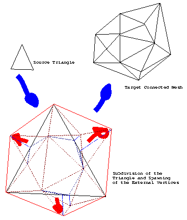
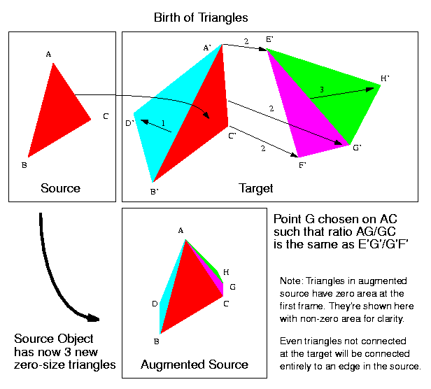
Spawning a vertex comes down to creating a zero-area triangle with two vertices shared with an existant edge of the nearest source triangle, and a third vertex at its middle (or some nicer ratio). Nicer ratio: suppose we need to place point A on an edge BC knowing that the whole will evolve into a triangle A'B'C'. We take the ratio A'B'/A'C', and we set A on BC such that it's the same as AB/AC. |
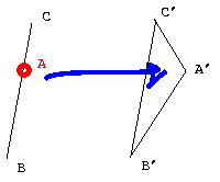 Figure 4: Spawning a vertex |
Assume (1) that the "many" triangles form a simply connected mesh: then we can find the external vertices of the mesh. Figure 5 shows an example of a triangle mapping to a connected mesh with 6 external vertices. We then map the vertices of the source triangle to the three that fit best (using nearest neighbors) of all those external vertices. The other external vertices will spawn off the edges of the source triangle, using the process described above, and marked on Figure 5 by bright blue (_._._._) lines. Now the shape of the mesh is created inside the virtual triangles formed by the vertices from the source triangle and the ones that are spawning from it: the shapes as they are formed at the beginning, when the spawning triangles are still flat, are shown in dark blue (.......) lines; the final shapes are in dark red (.......).
The challenges in this approach are: to assure assumption (1), that the mesh is simply connected; and to find the exterior vertices in a mesh.
We have to spawn off vertices on the outsides of the triangles and grow from their edge, as these edges move and morph. Since our program morphs linearly, a connected mesh at the arrival will be connected throughout its travel.
We spawn on the outside so that we don't destroy the "simplitude" of simple surfaces. If we spawn on the inside then we'd have to destroy the top edge from which the new triangles spawned, which cannot be done smoothly since those faces are huge.
The details on spawning (and a colorful figure!) are given later in this paper.
We could, in a more complicated version of the matching algorithm,
try spawning off triangles while keeping the entire mesh hole-less.
This would mean keeping vertices linked and letting triangles move as
their vertices do. However, this involves a radical changing of the
entire structure of our program, and we won't show interest in that at
this point in time, especially since we can't prove that all polygon
meshes are topologically similar, which means, they can be morphed
into each other, while all vertices remain shared, a claim which
seems easy to disprove by a counter example that will be left
as an exercise to the reader.
The matching process that we first considered would output a list
of exclusive one-triangle-to-many mappings that could then be
individually processed by one of the algorithms described above. The
special property of the "two-way" algorithm is that the one-to-many
mappings could go in both directions, from source to target as well as
from target to source, solving what Krzysztof called "the lollipop
problem":
|
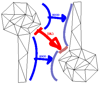
The Lollipop Problem: consider the "lollipop" on Figure 6, transforming into an object of similar shape in the opposite orientation: the object has two parts, with high and low triangle concentrations, respectively. Consider what happens when we use a matching algorihm that maps one-to-many only one way, i.e. the "one" comes from the object with less triangles, the "many" come from the object with more triangles, and if the two objects have the same number of triangles, it's a one-to-one mapping: some triangles in the high density parts of the source object will travel to the low density parts if those map to high density parts in the target object ("BAD" arrow). Instead we would want the triangles to stay locally, and create or destroy them as necessary ("GOOD" arrows). |
 |
This two-way matching process works as follows:
It seems to be quite a brute-force algorithm, but it guarantees a list of one-to-many mappings that solves the lollipop problem. Note: one way around the lollipop problem is by forcing the user to create two sub-objects for the lollipop: the candy (dense) and the stick (sparse) separate, and morph them separately into a stick and a candy, respectively.
Here are the problems with the approaches considered so far:
The problems with the shaping approach seemed impossible to overcome reasonably, and the algorithm itself is very hard to implement to begin with, hence we decided to drop it.
For the final program, we considered a new, more general approach, a more elaborate variant of the spawning process that uses a different matching process, and does not even assume that the objects are connected. It works around the lollipop problem by requiring the user to use separate sub-objects.
The morpher program has a feature which allows one to save the current frame as an image file, thus allowing the user to create a string of images which can be put together to make a movie. Open Inventor has a built in feature which saves an Inventor file as a .rgb file, thus allowing one to save still frames easily. It is easy to convert between image formats and Athena has a program that lets one create animated gifs which are little movies with morphing animations.
The off-screen renderer was actually not that difficult to implement because Inventor was nice and provided an OffScreenRenderer library which let me call the following routines to render an rgb file given an Inventor object:
  ...
  SoOffscreenRenderer *myRenderer =
    new SoOffscreenRenderer(myViewport);
  myRenderer->setBackgroundColor(SbColor(0,0,0)); /* black background */
  if (!myRenderer->render(root)) {
    delete myRenderer;
    return FALSE;
  }

  /* output .rgb file */
  FILE *fp = fopen(outputfile, "w");
  myRenderer->writeToRGB  (fp);
  ...
One little problem I experienced initially with the off-screen renderer was the requirement that the whole scene be under a single Separator node, but since our objects behaved this rule to begin with, it was not a problem. Another small problem with the OSR was that it also initially needed a camera and light position specified in separate files camera.iv and light.iv, but the Inventor libraries in C++ provide routines to dynamically get the camera and lighting information to produce a decent scene. Without this information, the OSR camera position may default to a position pointing away from the object, which would not be very useful.
After getting the OSR to work properly all the time, I incorporated the code as a procedure in the main morphing program and added a button on the main interface that will render the current scene immediately as an rgb file sceneX.rgb where X is the current frame number. The morpher keeps track of the current frame from 1 to N so the frames will be always saved in the correct order.
Thus when the morphing was done, there would be a bunch of files frame1.rgb, frame2.rgb, ..., frameN.rgb which needed to be strung together in a movie. There is a utility on Athena called whirlgif which takes a group of .gif files and makes an animated gif from them (which is easily viewable in Netscape or any other web browser).
The last issue that remained was to convert from .rgb to .gif and there was no converter available. However, doing "man rgb" showed a short 20 line C program on how to read a .rgb file and get its contents. Writing gifs is hard (because it involves a solid knowledge of LZW encoding and a lot of bit manipulation), but writing a .ppm is easy (it is just a string of red, green, blue values) and there is a utility on Athena to convert ppms to gifs, so combining all these tools, I wrote a little script called rgbtogif.
Now that I could make gifs from rgbs, I wrote a short script called makemovie which automatically senses all the files of the form frameX.rgb, converts them into gifs and strings them into an animated gif movie.
We want our morphing algorithm to have a natural user-friendly interface and also be interactive, requiring it to do graphics rendering on the fly. Originally, we thought about having a program to take in two sets of triangles each of a specific format because all of our morphing algorithms mapped triangles to triangles. However, if we wanted to have the morpher handle more complicated objects such as cubes, cylinders or spheres, we would have to first manually convert these to triangles to run them through the morpher.
Ideally, we wanted a program that would take objects of a high-level language (such as Inventor format), and morph them interactively. We then realized that in Assignment 4, we used a scan converter that took an OpenInventor file and automatically triangulized it. Using this, it was then easy to put these triangles into our data structures for the morphing algorithm. Since SceneViewer is easily extendible, we could write an extension of SceneViewer by adding a couple extra buttons to handle morphing interactively.
The interface we then decided on was to have the program read in a source and target Inventor files on the command line, bring up a SceneViewer window with added buttons "->" and "<-" to flip forward or backward through the stages of morphing. We set a morphing parameter k that went from 0 to N where k=0 is the source and k=N is the target and the other values represent intermediate scenes. Once all the geometry was calculated at the beginning and the nearest neighbor, all the mappings were completed, then creating intermediate scenes varying k was very fast. In fact, we could have SceneViewer render the intermediate scene on the fly, so as one repeatedly clicked the "->" button, he could see the object morphing continuously.
Later we added another option on the command line, which was the number of frames N or discrete steps k made. Large values made for smoother morphing with more frames. Finally we added a little button to do the off-screen rendering. When one clicks this button, the OSR would render the current scene, keeping track of the index k and rendering an image called "image(k).rgb".
We also included a -debug option on the command line which would print out a verbose report on all the steps the morpher went through so that if it had a problem, the problem could be pinpointed much easier. It is annoying to run a large program and all you see is "segmentation fault" and you have no idea where it broke. The -debug option also shows all the nearest neighbor calculations and how it matched vertices from the source to the target.
We're describing in this part the low-level algorithm to match m polygons to n polygons, without preserving any structure. Note that the structure in our structured morpher is obtained by calling this unstructured morphing algorithm iteratively on parts of the scene that the user has specified he/she wants to map to each other, as described earlier in this paper.
We'll also note that we're mapping objects which have been scaled and translated, such that their xyz bounding box is a unit cube centered at the origin.
Two techniques (shaping and spawning) were already presented for creating new polygons. The same techniques apply for making polygons disappear (since one can reverse source and destination environments when doing the matching to guarantee creation instead of deletion of polygons).
Consider however a morphing alorithm which has no cost assigned to those creations and deletions. In an extreme such case, the program would minimize to zero the old shapes, and create from zero the new shapes. We've taken all intelligence and progressivity out of morphing. We'll try and stay as far away from this as possible.
Thus, our main concern will be minimizing creation and deletion of polygons. Therefore we'll map as many polygons as we can in a one-to-one mapping, and only afterwards will we spawn off the rest as needed.
We'll start by examining the M-to-M mapping first, where m is the min number of polygons among the source and the target. We'll then introduce the Edge Ordering algorithm for doing such a mapping. Afterwards we'll examine the M to N mapping, and describe how new triangles spawn off in the scene. Finally we'll describe the Incremental Edge Ordering algorithm, an extension to our original Edge Ordering algorithm.
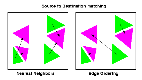
We'll use a nearest-neighbor type of algorithm to map the m objects into each other. A nearest-neighbor algorithm finds for each source the closest triangle in the target environment, and matches the two into each other, as shown in figure 7. In the next part we'll explain how we can obtain the match given by Edge Ordering, but first let's see why a nearest-neighbor approach makes sense.
The purpose is to create a one-to-one mapping with no creations and no deletions. Therefore we'll have to map as many as possible, which is what nearest neighbors is doing. Moreover, everything has been scaled to a cube of size 1, and therefore, distances can be used for mapping. Moreover, we don't want to try to be smart in the lowest level of the matching, since we've been smart earlier when matching nodes to nodes. We'll therefore match every polygon to its nearest on the other environment.
Definition of Nearest. We're here defining what we mean by distance between two triangles. Instead of the three-dimensional distance of triangle centers, which may seem an intuitive choice for the distance between two triangles, we'll choose the total straight-line distance travelled by all vertices of one polygon to become all vertices of the other polygon in an optimal permutation. In other words, we'll first look through all possible permutations of edges between two triangles (<1 2 3> can match to any of <1 2 3> <1 3 2> <2 1 3> <2 3 1> <3 1 2> <3 2 1>), and from those find the one which minimizes length traveled when going from one set of vertices to the other. Save that permutation (a number from 1 to 6) along with the optimal distance, the source and the destination in a data structure we'll call a match, since it's that permutation that we'll use if the two triangles end up matching. Let us add here that from those 6 permutations, three invert the normal and three don't. Therefore, we'll only use <1 2 3> <2 3 1> <3 1 2>, which don't invert the normal.
More precisely, instead of the sum of those distances, we'll use the sum of their squares. Reader will ask: why can we choose squares instead of distances themselves? Answer: coz 1) we don't have to take the square roots, 2) it gives a more balanced mapping. Illustration: For numbers greater than 1, it works intuitively, since the squares of large numbers are so much bigger than squares of smaller numbers. Example: sum of 1 10 1 is 12 in sum of distances, and 102 in sum of distances squared. However, 4 4 4 has a sum of distances of also 12, but a sum of squares of 48, which is largely smaller than 102. Therefore, for numbers greater than 1, a more balanced mapping would be chosen. Even though some may find it counter-intuitive, this reasoning also works for numbers which are all smaller than 1 (which is the case in our program, since we're scaling everything to a cube of size 1 when doing the mapping). Example, in the case of .01 .01 and .1, the sum of squares is .0102 while the sum of the numbers is .12. For the same sum .12 we could have .04 .04 and .04, in which case the sum of squares would become .0048, which is smaller than .0102, therefore the balanced thing will stll get chosen. A simple argument (convince yourselves, just like we did) is that we can scale everything by 1000 maintaining ratios, and since the scaling is uniform and can be eliminated in the inequality, we're still comparing squares of #'s bigger than 1. We'll therefore use sum of squares that yield more balanced travels.
However, a nearest-neighbor algorithm doesn't guarantee we'll have unique matches for each polygon, as one can see in figure 7. We'll call conflict a match which shares its source or its target with another match. An extended nearest neighbor would work if it has some way of resolving conflicts. It must either either resolve conflicts at the end, which can take a very long time and algorithms for which risk to be very complicated and recurse indefinitely, or if it can resolve conflicts incrementally, by mapping to the nearest polygon which is not already matched with another, in which case the algorithm is partial since it will match the nodes visited first without guaranteeing a globally optimal matching.
An alternative to a nearest-neighbor algorithm is the Edge Ordering Algorithm, introduced in 1997 by Manolis Kamvysselis, a junior in computer science at MIT. He originally used it for his final project in Computer Graphics, and we'll use it here, since it seems fit.
In this algorithm, each triangle is a node, and each matching between two triangles is an edge between two nodes. Since matchings are done only between the two non-intersecting spanning sets of sources and targets, the matching problem becomes the construction of a bipartite graph which connects all nodes, and each node only once.
The algorithm, illustrated in figure 8, is as follows:
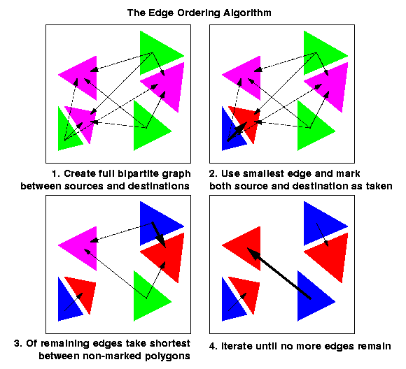
Correctness: When no more edges remain in our sorted list, we'll have achieved our bipartite graph. Proof: suppose at least one pair is unmatched. since our list contained an edge for every pair of nodes, it must have either not seen their edge (therefore we're not done, contradiction), or seen their edge and didn't connect them (therefore, one of the nodes must have been taken, therefore no unmatched pair of nodes exist).
Greedy strategy is optimal in polynomail time. The problem of finding the minimum length cycle in the full bipartite graph is NP hard, therefore, we can't wish to achieve an optimally optimal solution. However, our greedy approach does pretty well for its running time, since at each step it's adding the minimum weight edge available.
We assume we've already mapped m polygons to m others, and there remain n-m of them unmatched all in the same environment (by correctness argument) either in the source or in the target environment, without loss of generality.
We now have to spawn off additional triangles which have zero area in the source environment, but which will become good and healthy triangles in the target environment.
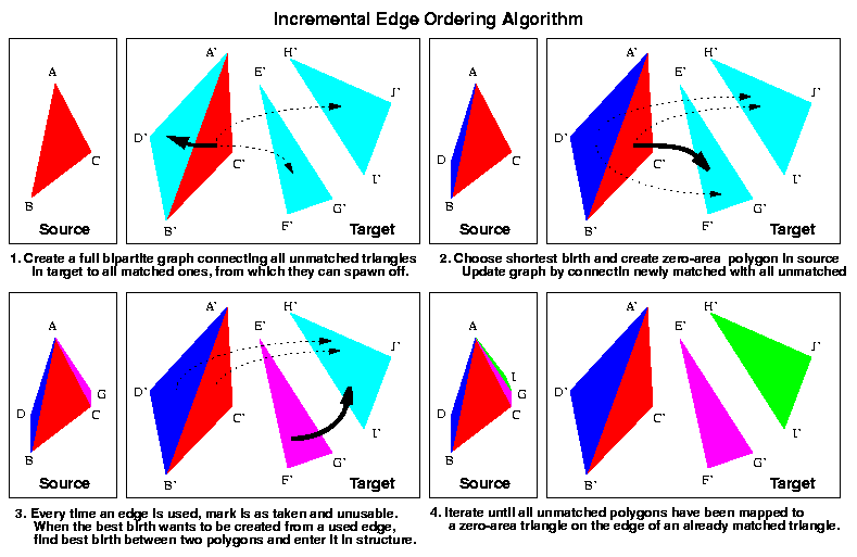
As illustrated in figure 8, for each unmatched triangle in the target environment, we'll look through the list of currently matched triangles in the target environment (the same environment this time), and we'll find the nearest edge from which to spawn the unmatched triangle. We'll then create a zero-area triangle on the corresponding edge of the corresponding triangle in the source environment (the edge from the source that'll become the best-birth edge in the target). The two endpoints will correspond to two endpoints, and the third will be created in the middle preserving the edge ratio described in the figure.
Measure of nearest. This time nearest edge is the one that minimizes the total length to be traveled from the target to the target were we to displace the triangle only in the target. The reason is that we want to keep a kind-of constant flow of triangles, and therefore we'll trust that the edge from which the triangle is spawned is already traveling right and doing the right thing, and we'll spawn off a triangle which will travel the least compared to that edge. It will travel the least, since it's starting on the edge, and it's finishing the closest to it than all other triangles. We now have to check more permutations for each triangle to be mapped. We'll also keep more information. We'll remember the parent triangle from which the unmatched triangle will spawn, the edge on that triangle from which it will spawn, the edge of the child triangle that will correspond to that edge, and the ratio of the two other edges. All that information will be kept in a structure we'll call a birth.
To do the m to n matching, we'll therefore use the following algorithm, illustrated in figure 9.
This algorithm sounds awefully expensive. We can't use the Kamvysselis Edge Ordering Algorithm, since it assumes the list of best edges does not get updated. It sorts it once, and keeps it so forever. We therefore would have to do an insertion sort if our data structure is a list.
To the rescue comes the Incremental Edge Ordering Algorithm, also developped in 1997 by Manolis Kamvysselis for his graphics final project. Same allegories, but this time we're sorting incrementally, hence the name Incremental Sorting Algorithm.
We'll keep a data structure containing the possible birth to be made between all matched triangles (and the best edge to use and the distance achieved by using the best edge), and all unmatched triangles.
The way to achieve such a functionality with an optimal time is a heap, a birth heap we'll call bheap. We insert in lg n time, and we extract the min in lg n time. The heap will contain all possible births between all matched polygons and all unmatched polygons.
The other problem is that the data inside our data structure is changing. When an edge is used to create one polygon, it cannot be used to create another. Therefore, if two unmatched polygons both had selected the same edge to be created from, as soon as one is selected, the other best birth will be invalid. It would be wrong to update every single best birth involving a polygon every time a birth is used with that polygon. Instead, we'll take care of such cases when trying to use a birth. If the mother edge is taken, we'll call best_birth again, with the same two polygons, only this time, it will consider the edge taken. When the match is made, we'll insert the node again in the heap.
The Incremental Edge Ordering Algorithm
Correctness: at any time, at least all possible births are included in the data structure, and the optimal one is handed in by the call to bheap_return_min. No impossible birth will be made between two polygons, since we're checking all criteria that would disallow the match. If, when the edge of a parent is already used, we're reconstructing a birth among those two polygons, we're guaranteed that it won't be better than any birth already used, since it's not better than the previous birth between those two polygons (otherwise, it would have been selected in the first time around), and the impossible birth is no better than any of the ones already used otherwise, it would have been extracted from the bheap earlier. Putting the new reconstructed birth and back, guarantees that if the birth leads to an optimal combination later on, it will get selected.
Greediness: by arguments above, at each step we're making the optimal choice for a birth. Finding the one best combination is however NP hard, and we're doing pretty well for a polygomial (times logarithmic) time.
The team would also like to express its gratitude towards our project supervisor, Luke Weisman, for his patience (when needed), impatience (when nothing else worked), and cool ideas.
We would also like to thank our friends, brothers, sisters, parents, roomates, pets, stuffed animals, and last but not least the TA's of other classes too, who supported our efforts of spending endless hours on this project. Thanks!
Finally, the team would like to thank the Anonymous Genius who wrote the IvScan. A lot of our knowledge about the Open Inventor as well as numerous parts of our code come from his work.