3.26 Space-time Poisson process Consider a highway that starts at x = 0 and extends infinitely eastward toward increasing values of x. Automobile accidents and breakdowns occur along the highway in a Poisson manner in time and space at a rate y per hour per mile. Any accident or breakdown that occurs remains at the location of occurrence until serviced.
    At time t = 0, when there are no unserviced accidents or breakdowns on the highway, a helicopter starts from     x = 0 flying eastward above the highway at a constant speed s. As a service unit, the helicopter will land at the site of any accident or breakdown that it flies over. Moreover, given at time t the helicopter is located at x = st, the helicopter can be dispatched (by radio) to service any accident or breakdown that occurs behind it (i.e., at values of x st). We assume that any such dispatch occurs immediately after the accident or breakdown occurs.
    We are interested in the time the helicopter first becomes busy, either by landing at an accident/breakdown site or by being dispatched to an accident/breakdown behind its current position; in the latter case, the instant of dispatch (not the time of arrival at the scene) is the time of interest.
    Let

T = time that the helicopter first becomes busy

a.

b. Let

probability that the first accident/breakdown is a dispatch incident behind the helicopter

1 - probability that the first accident/breakdown occurs as a result of patrol (i.e., the helicopter     discovers it)

Show that = 1 - = 1/2.

Hint: Condition on the event that the first accident breakdown occurs in the time interval (t, t + dt).

c. Let

X   location of the first accident/breakdown that the helicopter services

Show that

d. Suppose that

L₁, = time of first accident/breakdown that the helicopter flies over, assuming that it is no longer dispatched by radio (i.e., all incidents are helicopter-discovered incidents)

L₂ = time of first accident/breakdown that the helicopter is dispatched to, assuming that it never services accident/breakdowns that it flies over

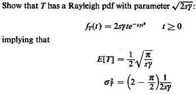
Then, for instance, T = Min[L₁, L₂]. Show that L₁ and L₂ are identically distributed Rayleigh random variables, each with parameter sy. Finally, argue that L₁ and L₂ are independent, thereby concluding that the minimum of two independent Rayleigh random variables, each with parameter  y, is itself a Rayleigh random variable with parameter  2y.

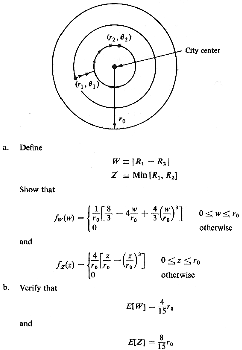
3.27 Circular city, revisited Suppose that two points (R₁, ₂) and (R₂, ₂) are independently, uniformly distributed over a circular city of radius r_o and area A= Suppose further that this city has a large number of radial routes and circular ring routes so that the travel distance between (R₁, ₁) and (R₂, ₂) can be accurately approximated as

D = |R1 - R2| + Min [ R1, R2] |₁ - ₂|

where 0 |₁ - ₂| signifies the magnitude of the angular difference between ₁ and ₂. In words, travel from an outer point, say, (R₁,₁) if R, > R2, to an inner point (R₂,₁) first occurs along a radial route to a ring located a distance R2 from the city center, and then along that ring (in the direction of minimum travel distance) to (R₂,₁); the same path is traveled in reverse if travel is from (R₂,₁) to (R₁,₁). A sample path is shown in Figure P3.27.

and thus

Compare this result to analogous results in Problems 3.20 and 3.21.

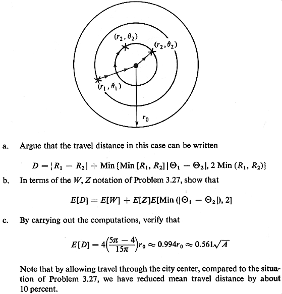
3.28 Circular city, revisited again Suppose we modify the previous example so that travel from the outer point to the inner point, when it reaches the inner circle (say of radius R₂ if R₂ < R₁), proceeds from that point either along an arc of radius R₂ (as in Problem 3.27) or through the city center along two radial routes directly to the possiblities are shown in Figure P3.28.

3.29 Effect of traffic lights on travel times  A vehicle travels a route from a to b, incurring a total travel time

T = 6 + W₁ + W₂   (minutes)

where     6 = time to traverse the distance (at constant speed) from a to b
           W₁ = delay incurred at traffic ight 1
           W₂ = delay incurred at traffic light 2

As shown in Figure P3.29, the route is partitioned into three 2-minute travel-time segments. Each traffic light operates on a fixed cycle of 1 minute green, followed by I minute red. (We assume that no time is wasted in decelerating and accelerating, should one or two lights cause the vehicle to stop.)

Suppose that exactly at some prespecified time (say 12: 00 noon) we examine the "phase"  _i, of each traffic light (i = 1, 2). By definition,

 _i = time until light i next turns to green (0 _i < 2)

For each light, we suppose that  _i, is independently, uniformly distributed over [0, 2]. However, once _i is known, its value isfixedfor all time.
    Throughout this problem, we assume that departure times at a occur independently of the phases of the traffic lights.

a. Find the mean and variance of the travel time from a to b.

b. Find the probability density function of the travel time from a to b.

c. Let k = number of traffic lights at which the vehicle is delayed. Find the z-transform of the probability mass function for k.

For parts (d) and (e), only [not for parts (f)-(h)], let

C = event that for the most recent vehicle traveling from a to b, the vehicle was stopped only at traffic light 1

d. Find the conditional joint probability density function for ₁ and ₂, given C.

e. Find the conditional probability density function for the travel time from a to b for the next vehicle to travel from a to b, given C. (Assume that you know nothing about when the next vehicle will leave a.)

For parts (f)-(h), suppose that vehicles leave a in a Poisson manner with mean = 1 vehicle per minute. Vehicles occupy zero space and, when in a traffic light queue, accelerate and decelerate instantaneously together.

f. Is the vehicle arrival process at b a Poisson process? Why or why not?

g. Determine the mean and variance of the queue length (number of vehicles) at traffic light I at the instant before the light turns green. (This is a primer for Chapter 4.)

h. A traffic engineer adjusts the phases of the two traflac lights so that ₁ = ₂ = 0 (relative to 12: 00 noon). Suppose that at 12: 00 noon we are given conditional information that no vehicles have left a during the last 8 minutes. Carefully sketch and label the probability density function for the time of arrival at b of the next vehicle to arrive there.

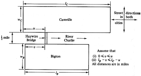
3.30 Expected travel distances in a two-city area Consider the cities of Camville and Bigton, which are separated by the River Charlie. Only the 1-mile-long Haywire Bridge connects the two towns. The layout of the cities is shown in Figure P3.30. The population of each of the two cities is uniformly distributed throughout the cities. Camville has a density of _c people per square mile; Bigton's density is _b people per square mile.

a. Find the expected travel distance between two randomly selected people in Camville; find the expected distance between two randomly selected people in Bigton.

b. Find the expected distance between a randomly selected person in Camville and a randomly selected person in Bigton.

C. Find the expected distance between two randomly selected people in the greater Camville-Bigton metropolitan area.

d. Find the expected distance between two randomly selected people, one from each town, assuming that one can cross the River Charlie at any point along the _B miles of Bigton that run along the river. By how much does your answer differ from your answer in part (b) ?

e. Compute numerical values for all the questions above assuming that
i. _B = 4 miles                               ii. _B = 2,000 people/square mile
   _c = 6 miles                                  _c = 1,000 peoplel/square mile
    u = 2 miles
     v = I mile
W_B = 5 miles
W_c = 3 miles

3.31 Assigning commuters to subway stations Figure P3.31 shows an urban area which is served only by a mass-transit rail line with four stops ~A, B, C, and D) as shown. There is a single destination at point T for all trips generated from this area (assume that all trips go exactly to point T) during each day's morning rush hour.

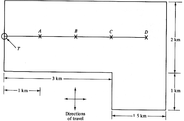
    In order to get to a transit line station or to walk directly to T, the residents of the area must walk on an "infinitely dense" grid of urban streets whose directions run parallel to the boundaries of the area.
    The following information is now given:

1. During the morning rush hour the area generates 200 trips per km^2 with trip origins distributed uniformly.

2. Headways between trains are constant and equal to 6 minutes, and each train rider is equally likely to arrive at a station at any time between two successive departures of trains from that station. (All riders are assumed to be able to ride on the first train to leave a station after their arrival there.) Stops at each station are I minute long.

3. Trains travel between stations at a speed of 30 km/hr (this includes an adjustment for acceleration and deceleration periods). People walk at a constant speed of 5 km/hr.

4. The sole criterion that each individual uses to determine his/her route is to minimize the expected total trip time to T (including time spent waiting for and riding on trains). Each individual is assumed to know all the information given above concerning travel speeds, headways, and so on.

a. Determine the number of riders who will be using each of stations A, B, C, and D each day, as well as the number of those that will be walking directly to T.

b. Compute the expected travel time for a random resident of this area each day.

c. Draw the boundary of the region whose residents are 9 minutes or less away from T. Repeat for the 20-minute boundary. (Be careful in your work.)

d. Repeat part (a) by making the change in the initial data indicated below, while keeping everything else the same as before. (Each part below is separate.)

1 . The train speed increases to 40 km/hr.

2. Train headways are increased to 10 minutes.

3. Train speed >> walking speed.

e. Repeat part (a) by assuming that headways between trains are described by a negative exponential pdf with a mean of 6 minutes.

3.32 Optimal district design in terms of city blocks In this problem we shall examine the question of optimal district design for cases in which the dimensions of a district can assume only integer values due to the grid structure of streets.
    Consider again the case described in Problem 3.15, which involved an n x m rectangular grid district with two-way streets. In that problem you have shown that

    Suppose now that we wish to design a district so as to minimize E[D], subject to the constraint that the area of the district is greater than or equal to some value A (i.e., mn A). (It is not reasonable to set an equality constraint since m and n can take only integer values.) For instance, if A = 44, we wish to find n and m such that E[D] is minimized and the district contains at least 44 city blocks.

a. Consider the quantity

under the constraint n + m = C (where C is a positive integer constant). Argue that under this constraint Q is maximized when n = m (if C is an even number) or n = m + I (if C is an odd number), and minimized when n = 0 or when m = 0.

Hint: Q is symmetric in n and m.

b. Show that the following algorithm will give the optimal district dimensions [LARS 72a]:

STEP 1: Set i = [A], where [x] = smallest integer greater than or equal to x.

STEP 2: Set j = i - 1 if i(i - 1) A; otherwise, set j =  i.

STEP 3: Set k = i + 1, = j - 1.

STEP 4: If kt A, set i = k, j = 1; return to Step 3. Otherwise, stop; the optimal district dimensions are n = i,
              m = j.

c. Apply your algorithm to find the optimal district dimensions for the case A = 44.

d. Compare numerically E[D] for the cases: m = 7, n = 7; m = 6, n = 8; m = 5, n = 9; m = 4, n = 11. (All these designs satisfy mn 44.) What do you conclude from these numerical comparisons?