3.9 Functions of random variables (derived distributions) Consider a square service region of unit area in which travel is right-angle and directions of travel are parallel to the sides of the square. Let (X₁, Y₁) be the location of a mobile unit and (X₂, Y₂) the location of a demand for service. The travel distance is

D = D_x + D_y

where

D_x = |X₁ - X₂| and D_y = |Y₁ - Y₂|

We assume that the two locations are independent and uniformly distributed over the square.

3.10 Ratio of right-angle and Euclidean travel distances In this problem we test the reasonableness of the isotropy assumption used in Example 4. It is appropriate to question this assumption since most service regions in a city are such that will not be uniformly distributed between 0 and /2. We consider three cases.

b. Case 2. Suppose that the square-unit-area service area of part (a) is rotated at a 45° angle to the directions of travel. In such a case intuition might lead one to think that E[R] would be less than 4/. Why? To investigate this conjecture it is helpful to use the relationship

where the primed variables are defined relative to a coordinate system rotated at 45° with respect to the original coordinate system. Show that in such a case

(Intuition is correct but the result is closer to 4/ than might otherwise have been expected.)

C. Case 3. Suppose that the mobile unit is located uniformly on the perimeter of a square rotated at 45° to the directions of travel. Suppose that the unit travels in a shortest (right-angle) distance manner to the center of the square. Again, T is the angle at which the directions of travel are rotated with respect to the straight line connecting the unit's initial position to the center of the square. Show that

Do all the results for E[R] check with your intuition?

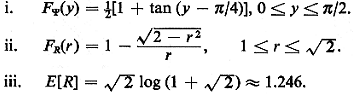
3.11 Quantization model (continued) In Example 5 we described a quantization model for odometer readings. We stated that [(3.31)]

    Prove these results. What implications do these results have for an actual datagathering experiment?

Hint: Do not work directly with (3.30); instead, demonstrate the validity of the desired results for any {D = d} and then integrate over all d.

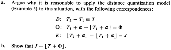
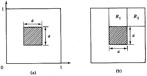
3.12 Truncated times Assume that an activity commences at time T₁ and terminates at time T₂. The exact duration of the activity is T₂ - T₁, T. Now assume that times are recorded by some mechanism that records time x as     [x+], for some fixed . Using this mechanism, the recorded duration of the activity is. [T₂ + ] - [T₁ + ].

3.13 Zero-demand zone Consider a unit-square response area, as shown in Figure P3.13(a). We assume that a response unit and incident (i.e., requests for service) are distributed uniformly, independently over that part of the unit square not contained within the central square having area a₂. Travel occurs according to the right-angle metric, and travel is allowed through the zero-demand zone. 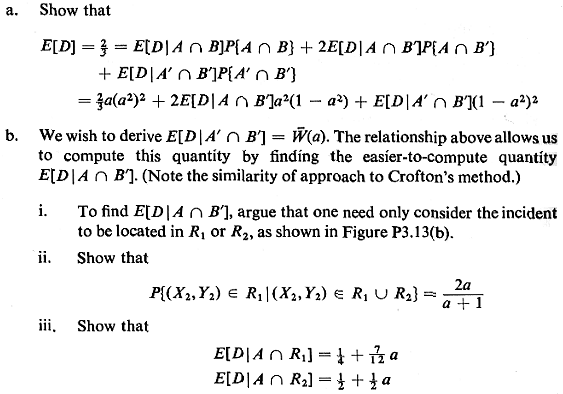We want to use conditioning arguments to derive the expected travel distance W(a) to a random incident.
    Let (X₁, Y₁) and (X₂, Y₂) denote the locations of the response unit and incident, respectively. Let S (S') denote the set of points within (outside) the central square.

    Now focus on a unit square on which incidents and the response unit are uniformly, independently distributed over the entire square, yielding an expected travel distance E[D].

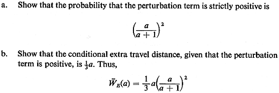
c. Finally, find W(a). As a check, W(0) = 2/3, W(1) = 11/12. (Why?)

3.14 Square barrier Suppose that the conditions of Problem 3.13 apply, except that in addition, no travel is allowed through the central square. We wish to derive

W'(a) = expected travel distance to a random incident

We use perturbation arguments to write

W"(a) = W(a) + W_E,(a)

where W(a) is the mean travel distance from Problem 3.13 and W_E(a) is the mean extra (perturbation) distance due to the barrier.

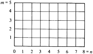
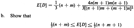
As a check, verify the reasonableness of the result W'(l) = 1.

3.15 Rectangular grid of two-way streets Consider an n x m rectangular grid of two-way streets running north-south and east- west as shown in Figure P3.15. Assume that incident positions are distributed uniformly over the grid. A response unit patrols the grid in a uniform manner. The incident location and the response unit location are independent. Let

D = travel distance between the response unit and the incident, assuming the unit follows a shortest path that remains on the streets of the grid

a. (Optional) By carefully and patiently conditioning on the various possible locations for the incident and response unit, show that

where the left-hand inequality becomes an equality when n or m is zero and the right-hand inequality becomes an equality when n = m. Thus, the continuous approximation, (3.12a), is never in error by more than I block length.

3.16 Perturbation variables: one-way streets Consider a very large grid of equally spaced one-way streets, with the direction of travel alternating from street to adjacent parallel street. Assume that the positions of the response unit and the incident are independent and uniformly distributed over the grid. It is assumed that the response distance -from the response unit to the incident is a shortest path that remains on the streets of the grid and obeys the one-way constraints. Use perturbation variables to demonstrate that the mean extra distance traveled to the incident, due to the one-way travel constraints, is two blocks.