 (I.1)
(I.1)A VISUAL TOUR OF CLASSICAL ELECTROMAGNETISM
Produced by
The TEAL/Studio Physics Project
Massachusetts Institute of Technology
For The MIT Course
Physics 8.02: Electromagnetism I
A. Scalar Fields and How We Represent Them
1. Sources and Sinks In Fluid Flows
3. The Relationship Between Fluid Flow Fields and Electromagnetic Fields
C. How We Represent Electromagnetic Vector Fields
1. The “Vector Field” Representation of A Vector Field
2. The “Field Line” Representation Of A Vector Field
3. “Grass Seeds” and “Iron Filings” Representations
A. Coulomb’s Law and Faraday’s Lines of Force
2. The Electric Field Of A Point Charge And Of A Collection Of Point Charges
3. Examples of Electric Fields Due To A Collection Of Charges
C. Stresses Transmitted by Electric Fields
2. Examples of Stresses Transmitted By Fields In Electrostatics
a) A Charged Particle Moving In A Constant Electric Field
b) A Charged Particle At Rest In A Time-Changing External Field
E. Electric Fields Hold Atoms Together
1. The Magnetic Field Of A Moving Point Charge And Of A Current Element
2. The Magnetic Fields Of Charges Moving In A Circle
a) Animations of the Magnetic Fields of 1, 2, 4, and 8 Charges Moving In A Circle
b) A ShockWave Simulation of the Magnetic Field Of A Ring Of Moving Charges
B. Stresses Transmitted By Magnetic Fields
2. Examples of Stresses Transmitted By Magnetic Fields
a) A Charged Particle Moving In A Time-Changing External Magnetic Field
b) A Charged Particle Moving In A Constant Magnetic Field
c) Forces Between Current Carrying Parallel Wires
d) Forces Between Co-axial Current-Carrying Circular Wire Loops
A. Time Changing Magnetic Fields Are Always Associated With Electric Fields
“… In order therefore to appreciate the requirements of the science [of electromagnetism], the student must make himself familiar with a considerable body of most intricate mathematics, the mere retention of which in the memory materially interferes with further progress …”
James Clerk Maxwell [1855]
Classical electromagnetic field theory emerged in more or less complete form in 1873 in James Clerk Maxwell’s A Treatise on Electricity and Magnetism. Maxwell based his theory in large part on the intuitive insights of Michael Faraday. The wide acceptance of Maxwell’s theory has caused a fundamental shift in our understanding of physical reality. In this theory, electromagnetic fields are the mediators of the interaction between material objects. This view differs radically from the older “action at a distance” view that preceded field theory.
What is “action at a distance”? It is a world view in which the interaction of two material objects requires no mechanism other than the objects themselves and the empty space between them. That is, two objects exert a force on each other simply because they are present. Any mutual force between them (for example, gravitational attraction or electric repulsion) is instantaneously transmitted from one object to the other through empty space. There is no need to take into account any method or agent of transmission of that force, or any finite speed for the propagation of that agent of transmission. This is known as “action at a distance” because objects exert forces on one another (“action”) with nothing but empty space (“distance”) between them. No other agent or mechanism is needed.
Many natural philosophers objected to the “action at a distance” model because in our everyday experience, forces are exerted by one object on another only when the objects are in direct contact. In the field theory view, this is always true in some sense. That is, objects that are not in direct contact (objects separated by apparently empty space) must exert a force on one another through the presence of an intervening medium or mechanism existing in the space between the objects.
The force between the two objects is transmitted by direct “contact” from the first object to an intervening mechanism immediately surrounding that object, and then from one element of space to a neighboring element, in a continuous manner, until it is transmitted to the region of space contiguous to the second object, and thus ultimately to the second object itself.
Although the two objects are not in direct contact with one another, they are in direct contact with a medium or mechanism that exists between them. The force between the objects is transmitted (at a finite speed) by stresses induced in the intervening space by the presence of the objects. The “field theory” view thus avoids the concept of “action at a distance” and replaces it by the concept of “action by continuous contact”. The “contact” is provided by a stress, or “field”, induced in the space between the objects by their presence.
This is the essence of field theory, and is the foundation of all modern approaches to understanding the world around us. Classical electromagnetism was the first field theory. It involves many concepts that are mathematically complex. As a result, even now it is difficult to appreciate. The purpose of this “visual tour” of electromagnetism is to impart a flavor of the essence of this theory using visual imagery.
A field is a function that has a different value at every point in space. A scalar field is a field for which there is a single number associated with every point in space. A good example of this is the temperature of the Earth’s atmosphere at the surface. Another example is the analytic expression
(I.1)
This expression defines the value of the scalar function ![]() at
every point
at
every point ![]() in space.
in space.
How do visually represent a scalar field defined by
an equation like the one in equation (I.1)? One way is to fix
one of our independent variables (z, for example) and then show a contour
map for the two remaining dimensions, in which the curves represent lines of
constant values of the function ![]() . A
series of these maps for various (fixed) values of z then will give a
feel for the properties of the scalar function. We show such a
contour map in the xy plane at z = 0 for equation (I.1).
Various contour levels are shown in Figure 1, labeled by the value of
the function at that level.
. A
series of these maps for various (fixed) values of z then will give a
feel for the properties of the scalar function. We show such a
contour map in the xy plane at z = 0 for equation (I.1).
Various contour levels are shown in Figure 1, labeled by the value of
the function at that level.
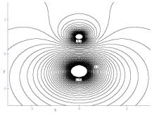
Figure 1: A contour map in the xy plane of electric potential given by equation (I.1).
Another way we can represent the values of the scalar
field is by color-coding in two dimensions for a fixed value of the third. Figure
2 shows such a map for equation (I.1), again at z = 0. Different
values of the function ![]() are
represented by different colors in the map.
are
represented by different colors in the map.
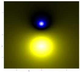
Figure 2: A color-coded map in the xy plane of electric potential given by equation (I.1).
A third way to represent a scalar field is to fix one of the dimensions, and then plot the value of the function as a height versus the remaining spatial coordinates, say x and y, that is, as a relief map. Figure 3 shows such a map for the function in equation (I.1), assuming z = 0.
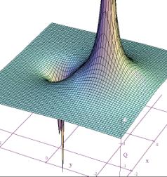
Figure 3: A relief map of the function given in equation (I.1) for z = 0.
A vector field is a field in which there is a vector associated with every point in space—that is, three numbers instead of only the single number for the scalar field. An example of a vector field is the velocity of the Earth’s atmosphere, that is, the wind velocity. Since fluid flows are the easiest vector fields to visualize, we first show examples of these kinds of vector fields
In Figure 4 we show a physical example of a fluid flow field, where we represent the fluid by a finite number of particles to show the structure of the flow. In this Figure, particles (fluid elements) magically appear at the center of a cone (a “source”) and then flow downward under the effect of gravity. That is, we are creating particles at the origin, and they subsequently flow away from their creation point. We also call this a diverging flow, since the particles appear to “diverge” from the creation point. In Figure 5 we show the converse of this, a converging flow, or a “sink” of particles.
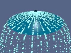
Figure 4: An example of a source of particles and the flow associated with a source.

Figure 5: An example of a sink of particles and the flow associated with a sink.
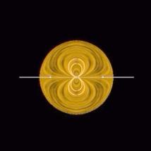
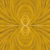
In Figure 6 we show another representation of a diverging flow. Here the direction of the flow is represented by a texture pattern in which the direction of correlation in the texture is along the field direction. Figure 7 shows a source next to a sink of lesser magnitude. Figure 8 shows two sources of unequal strength.

Figure 6: Representing the flow field associated with a source using textures.

Figure 7: The flow field associated with a source and a sink where the sink is smaller than the source.
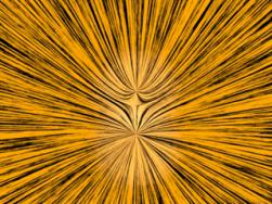
Figure 8: The flow field associated with two sources of unequal strength.
Finally, in Figure 9, we show a constant downward flow interacting with a diverging flow. The diverging flow is able to make some headway “upwards” against the downward constant flow, but eventually turns and flows downward, overwhelmed by the strength of the “downward” flow.
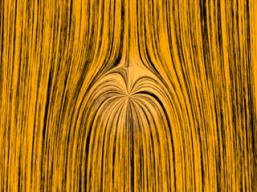
Figure 9: A constant downward flow interacting with a diverging flow.
In Figure 10 we show a physical example of a flow field that is neither a source or a sink—the flow is simply circulating. Particles are not created or destroyed (except at the beginning of the animation), they simply move in circles. In Figure 11 we show another way of representing a purely circulating flow using textures, similar to Figure 6.
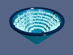
Figure 10: An example of a circulating fluid.

Figure 11: Another way of representing a circulating flow.
In Figure 12 we show a flow field that has two systems of circulation centered about different points in space. The circulating flows are in opposite senses, and one of the circulations is stronger than the other. In Figure 13 we have the same situation, except that now the two circulations are in the same sense.

Figure 12: A flow with two circulation centers with opposite directions of circulation.

Figure 13: A flow with two circulation centers with the same direction of circulation.
Finally, in Figure 14, we show a constant downward flow interacting with a circulating flow. The circulating flow is able to make some headway against the downward constant flow, but eventually is overwhelmed by the strength of the “downward” flow.
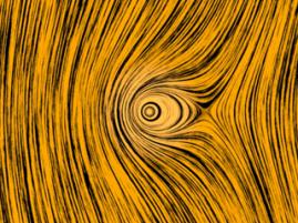
Figure 14: A constant downward flow interacting with a circulating flow.
In the language of vector calculus, the flows shown in Figures 10 through 14 are said to have a non-zero curl, but zero divergence. In contrast, the flows shown in Figures 6 through 9 have a zero curl (they do not move in circles) and a non-zero divergence (particles are created or destroyed).
Finally, in Figure 15, we show a fluid flow field that has both a circulation and a divergence (both the divergence and the curl of the vector field are non-zero). Any vector field can be written as the sum of a curl-free part (no circulation) and a divergence-free part (no source or sink). We will find in our study of electromagnetism that in statics, the electric fields are curl free (e.g. they look like Figures 6 through 9) and the magnetic fields are divergence free (e.g. they look like Figures 11 through 13). It is only when we come to time-varying situations that we will see electric fields that have both a divergence and a curl, that is that look like the field in Figure 15. As far as we know, even in time-varying situations magnetic fields are always divergence free. That is, magnetic fields will always look like the patterns we show in Figures 11 through 14.

Figure 15: A fluid flow field that has both a source and a circulation.
Vector fields that represent fluid flow have an immediate physical interpretation: the vector at every point in space represents a direction of motion of a fluid element, and we can construct animations of those fields, as above, which show that motion. A more general vector field, for example the electric and magnetic fields discussed below, do not have that immediate physical interpretation of a flow field. There is no “flow” of a fluid along an electric field or magnetic field.
However, even though the vectors in electromagnetism do not represent fluid flow, we carry over many of the terms we use to describe fluid flow to describe electromagnetic fields as well. For example we will speak of the flux (flow) of the electric field through a surface. If we were talking about fluid flow, “flux” would have a well-defined physical meaning, in that the flux would be the amount of fluid flowing across a given surface per unit time. There is no such meaning when we talk about the flux of the electric field through a surface, but we still use the same term for it, as if we were talking about fluid flow. Similarly we will find that magnetic vector field exhibit patterns like those shown above for circulating flows, and we will sometimes talk about the circulation of magnetic fields. But there is no fluid circulating along the magnetic field direction.
We use much of the terminology of fluid flow to describe electromagnetic fields because it helps us understand the structure of electromagnetic fields intuitively. However, we must always be aware that the analogy is limited.
Now let us turn from fluid flow to more general vector fields. Because there is much more information to represent in a vector field, our visualizations are correspondingly more complex when compared to the representations of scalar fields. Let us introduce an analytic form for a vector field and discuss the various ways that we represent it.
 (I.2)
(I.2)
This field is proportional to the electric field of two point charges of opposite
signs, with the magnitude of the positive charge three times that of the negative
charge. The positive charge is located at ![]() and
the negative charge is located at
and
the negative charge is located at ![]() .
We discuss how this field is calculated in a later section.
.
We discuss how this field is calculated in a later section.
Figure 16 is an example of a “vector field” representation of equation (I.2), in the plane where z = 0. We show the charges that would produce this field if it were an electric field, one positive (the orange charge) and one negative (the blue charge). We will always use this color scheme to represent positive and negative charges.
In the vector field representation, we put arrows representing the field direction on a rectangular grid. The direction of the arrow at a given location represents the direction of the vector field at that point. In many cases, we also make the length of the vector proportional to the magnitude of the vector field at that point. But we also may show only the direction with the vectors (that is make all vectors the same length), and color-code the arrows according to the magnitude of the vector. Or we may not give any information about the magnitude of the field at all, but just use the arrows on the grid to indicate the direction of the field at that point.
Figure 16 is an example of the latter situation. That is, we use the arrows on the vector field grid to simply indicate the direction of the field, with no indication of the magnitude of the field, either by the length of the arrows or their color. Note that the arrows point away from the positive charge (the positive charge is a “source” for electric field) and towards the negative charge (the negative charge is a “sink” for electric field).
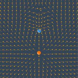
Figure 16: A “vector field” representation of the field of two point charges, one negative and one positive, with the magnitude of the positive charge three times that of the negative charge. In the applet linked to this figure, one can vary the magnitude of the charges and the spacing of the vector field grid, and move the charges about.
There are other ways to represent a vector field. One of the most common is to draw “field lines”. Faraday also called these “lines of force”. To draw a field line, start out at any point in space and move a very short distance in the direction of the local vector field, drawing a line as you do so. After that short distance, stop, find the new direction of the local vector field at the point where you stopped, and begin moving again in that new direction. Continue this process indefinitely. Thereby you construct a line in space that is everywhere tangent to the local vector field. If you do this for different starting points, you can draw a set of field lines that give a good representation of the properties of the vector field. Figure 17 below is an example of a field line representation for the same two charges we used in Figure 16.
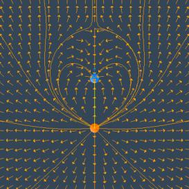
Figure 17: A “vector field” representation of the field of two point charges, and a “field line” representation of the same field. The field lines are everywhere tangent to the local field direction
The final representation of vector fields is the “grass seeds” representation or the “iron filings” representation. For an electric field, this name derives from the fact that if you scatter grass seeds in a strong electric field, they will orient themselves with the long axis of the seed parallel to the local field direction. They thus provide a dense sampling of the shape of the field. Figure 18 is a “grass seeds” representation of the electric field for the same two charges in Figures 16 and 17. The local field direction is in the direction in which the texture pattern in this figure is correlated. This “grass seeds” representation gives by far the most information about the spatial structure of the field.
We will also use this technique to represent magnetic fields, but when used to represent magnetic fields we call it the “iron filings” representation. This name derives from the fact that if you scatter iron filings in a strong magnetic field, they will orient themselves with their long axis parallel to the local field direction. They thus provide a dense sampling of the shape of the magnetic field.
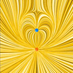
Figure 18: A “grass seeds” representation of the electric field that we considered in Figures 16 and 17. In the applet linked to this figure, one can generate “grass seeds” representations for different amounts of charge and different positions.
A frequent question from the student new to electromagnetism is “What is between the field lines?” Figures 17 and 18 make the answer to that question clear. What is between the field lines are more field lines that we have chosen not to draw. The field itself is a continuous feature of the space between the charges.
In what follows we will show the spatial structure
of electromagnetic fields using all of the methods discussed above. In
addition, for the field line and the grass seeds and iron filings representation,
we will frequently show the time evolution of the fields. We do
this by having the field lines and the grass seed patterns or iron filings patterns
move in the direction of the energy flow in the electromagnetic field at a given
point in space. This direction is in the ![]() direction, and
is perpendicular to both E and B. This is very different
from our representation of fluid flow fields above, where the direction of the
flow is in the same direction as the velocity field itself.
direction, and
is perpendicular to both E and B. This is very different
from our representation of fluid flow fields above, where the direction of the
flow is in the same direction as the velocity field itself.
We adopt this representation for time-changing electromagnetic fields because these fields can both support the flow of energy and can store energy as well. We will discuss quantitatively how to compute this energy flow later. For now we simply note that when we animate the motion of the field line or grass seeds or iron filings representations, the direction of the pattern motion indicates the direction in which energy in the electromagnetic field is flowing.
In Maxwell’s theory, electromagnetic fields are the mediators of the interaction between material objects. As we pointed out above, this view differs radically from the older “action at a distance” view. To illustrate the difference between the field approach and the “action at a distance” approach, we introduce Coulomb’s Law.
Coulomb’s Law
There are two kinds of electric charge, which we denote as positive and negative. Like electric charges attract, and unlike electric charges repel, with a force that is inversely proportional to the square of the distance between them and directly proportional to the product of their charges. In equations, the magnitude of the force F is give by
![]() (II.1)
(II.1)
where ![]() is
a constant.
is
a constant.
This statement of Coulomb’s Law on the face of it sounds like “action at a distance”. There is no reference to any intervening mechanism for transmitting the force between the charges. The force simply exists because the particles are there, and there is no reference to a field. But it is precisely the intervening “electric field” between the two charges that is the mechanism by which the force in equation (II.1) is transmitted.
To demonstrate what we mean by this, consider Figure 19. This figure illustrates the repulsive force transmitted between two objects by their electric fields. One object is the charged metal sphere of a van de Graaff generator. This sphere is fixed in space and is not free to move. The other object is a small charged sphere that is free to move (we neglect the force of gravity on this sphere). According to Coulomb’s Law, these two like charges repel each another. That is, the small sphere feels a repulsive force away from the van de Graaff sphere. The animation shows the motion of the small sphere and the electric fields in this situation. To make the motion of the small sphere repeat in the animation, we have the small sphere “bounce off” of a small square fixed in space some distance from the van de Graaff.
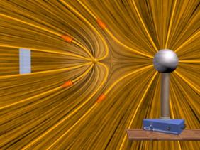
Figure 19: Two charges of the same sign that repel one another because of the stresses transmitted by electric fields. We use both a “grass seeds” representation and a ”field lines” representation of the electric field of the two charges.
Before we discuss this animation, consider Figure 20, which shows one frame of a movie of the interaction of two charges with opposite signs. Here we have given the small sphere an electric charge that is opposite to that on the van de Graaff sphere. According to Coulomb’s Law, the two objects now attract one another. That is, the small sphere always feels a force attracting it toward the van de Graaff. To make the motion of the small sphere repeat in the animation, we have that charge “bounce off” of a square fixed in space near the van de Graaff.
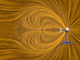
Figure 20: Two charges of opposite sign that attract one another because of the stresses transmitted by electric fields.
The point of these two animations is to underscore the fact that the Coulomb force between the two charges is not “action at a distance”. Rather, the stress is transmitted by direct “contact” from the van de Graaff to the immediately surrounding space, via the electric field of the charge on the van de Graaff. That stress is then transmitted from one element of space to a neighboring element, in a continuous manner, until it is transmitted to the region of space contiguous to the small sphere, and thus ultimately to the small sphere itself. Although the two spheres are not in direct contact with one another, they are in direct contact with a medium or mechanism that exists between them. The force between the small sphere and the van de Graaff is transmitted (at a finite speed) by stresses induced in the intervening space by their presence.
Michael Faraday invented field theory, and his drawing of “lines of force” or “field lines” was his way of representing the fields. He also used his drawings of the lines of force to gain insight into the stresses that the fields transmit. He was the first to suggest that these fields, which exist continuously in the space between charged objects, transmit the stresses that result in forces between the objects.
Faraday thought of the repulsive force in Figure 19 as due to a “push” or “pressure” exerted perpendicular to his lines of force. When the small sphere is moving closer to the van de Graaff and slowing down, its kinetic energy is being stored in the field as the field is compressed, just as a spring stores energy as it is compressed. When the small sphere is moving away from the van de Graaff and speeding up, it does so because energy that was stored in the field in the previous compression is now being converted back into the kinetic energy of the small sphere. Thus, Faraday’s “field” not only enables the transmission of force between the two objects, but it stores energy as well.
In contrast, Faraday thought of the attractive force in Figure 20 as due to a “pull” or “tension” exerted along his lines of force. When the small sphere is moving away from the van de Graaff and slowing down, its kinetic energy is being stored in the field as that field is “stretched”, just as a spring stores energy as it is stretched. When the small sphere is moving back toward the van de Graaff and speeding up, it does so because the energy that was stored in the field in the previous stretching is now being converted back into the kinetic energy of the moving object. In both Figures 19 and 20, the motion of the field indicates the direction of the flow of energy in the fields. That flow is from the particle’s kinetic energy to the field as the particle slows, and from the field back to the particle’s kinetic energy, as the particle speeds up.
It was Faraday’s “lines of force” model that Maxwell embraced in his Treatise on Electricity and Magnetism. In Maxwell’s words,
“…Faraday, in his mind’s eye, saw lines of force traversing all space where the mathematicians saw centres of force attracting at a distance. Faraday saw a medium where they saw nothing but distance. Faraday sought the seat of the phenomena in real actions going on in the medium, they were satisfied that they had found it in a power of action at a distance impressed on the electric fluids.”
James Clerk Maxwell [1873]
To move beyond the qualitative descriptions above, we now define the electric
field quantitatively. We do this in terms of forces on a test
charge. Let qtest be a test charge.
To find the electric field at some point in space (x,y,z), we
place the test charge at that point in space and measure the force
![]() on the test
charge. Then the electric field is found by taking the limit
on the test
charge. Then the electric field is found by taking the limit
The Electric Field
![]() (II.2)
(II.2)
Comparing (II.1) with (II.2), we see that the electric field of a point charge with charge q is given by
The Electric Field Of A Point Charge
![]() (II.3)
(II.3)
where r is the distance between the charge and the observation point
at which the field is being measured, and the unit vector ![]() points
from the source of the field (the charge) to
the observation point.
points
from the source of the field (the charge) to
the observation point.
Figure 21 is an interactive ShockWave display that shows the electric field of a positive point charge computed from equation (II.3). This interactive display allows you to move the position of the observer about the source charge to see how moving that position changes the magnitude and direction of the electric field at the observer.
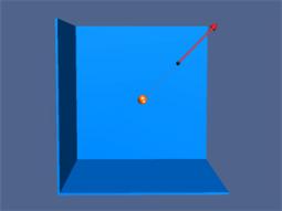
Figure 21: The electric field of a positive point charge points from the charge to the observation point.
Finally, to show another visualization of the electric field of a point charge, Figure 22 and Figure 23 show one frame of animations of the electric field of a moving positive and negative point charge, assuming the speed of the charge is small compared to the speed of light.
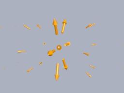
Figure 22: The electric field of a moving positive charge when the speed of the charge is small compared to the speed of light.
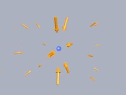
Figure 23: The electric field of a moving negative charge when the speed of the charge is small compared to the speed of light.
To find the field of a collection of point charges, we simply sum up the fields due to each of the charges it the collection. This is the Principle of Superposition.
The Electric Field Of A Collection Of Point Charges
Consider a collection of point charges ![]() for
i = 1 to N. Let the ith charge be located in space
at
for
i = 1 to N. Let the ith charge be located in space
at ![]() . Then
the electric field at a point
. Then
the electric field at a point ![]() is given by
is given by
 (II.4)
One of the most important field configurations we will study is that of the electric dipole. This is the field pattern created by two charges with opposite signs of charge. If the magnitude of both of the charges is q, and the electric charges are separated by a distance d, then the electric dipole moment p points from the negative charge to the positive charge and has magnitude qd. Figure 24 shows the field lines of this charge configuration.
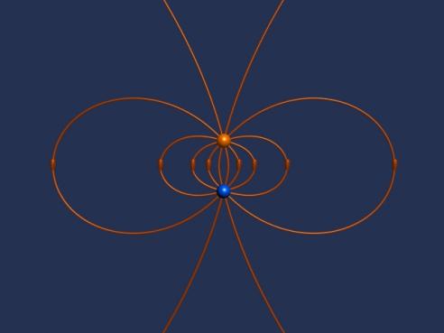
Figure 24: The electric field lines of two opposite charges close together.
Another way to represent this field is to use a simulation that shows how the electric fields of the individual charges add up to give the dipole pattern. Figure 25 shows an interactive ShockWave simulation of how the dipole pattern arises. At the observation point, we show the electric field due to each charge, which sum vectorially to give the total field. To get a feel for the total electric field, we also show a “grass seeds” representation of the electric field in this case. We can move the observation point around in space to see how the resultant field at various points arises from the individual contributions of the electric field of each charge.
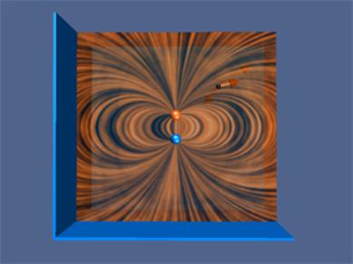
Figure 25: An interactive ShockWave simulation of the electric field of an two equal and opposite charges.
Suppose we want to calculate the electric field of a large number of charges, say 20 equal charges sitting arranged on a line with equal spacing between the charges. To calculate this field we have to add up vectorially the electric fields of each of the 20 charges. Figure 26 shows a ShockWave display of this vectoral addition at a fixed observation point. As the addition proceeds, we also show the resultant up to that point (large arrow in the display).
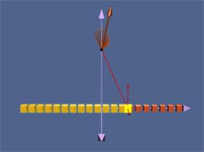
Figure 26: A simulation of the use of the principle of superposition to find the electric field due to a finite line of charges at a fixed observation point.
In Figure 27, we show an interactive ShockWave display that is similar to that in Figure 26, but now we can interact with the display to move the position of the observer about in space. To get a feel for the total electric field, we also show a “grass seeds” representation of the electric field due to these charges. We can move the observation point about in space to see how the resultant field at various points arises from the individual contributions of the electric field of each charge.
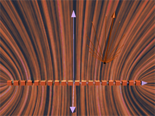
Figure 27: An interactive simulation of the calculation of the electric field due to a finite line of charges. We can move the observation point about to see the resultant field at different points in space.
Suppose we want to calculate the electric field of a large number of charges, say 30 equal charges, arranged on the circumference of a circle with equal spacing between the charges. To calculate this field we have to add up vectorially the electric fields of each of the 30 charges. Figure 28 shows a ShockWave display of this vectoral addition at a fixed observation point on the axis of the ring. As the addition proceeds, we also show the resultant up to that point (large arrow in the display).
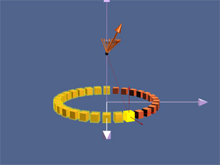
Figure 28: A simulation of the use of the principle of superposition to find the electric field due to 30 charges arranged in a ring at an observation point on the axis of the ring.
In Figure 29, we show an interactive ShockWave display that is similar to that in Figure 28, but now we can interact with the display to move the position of the observer about in space. To get a feel for the total electric field, we also show a “grass seeds” representation of the electric field due to these charges. We can move the observation point about in space to see how the resultant field at various points arises from the individual contributions of the electric field of each charge.
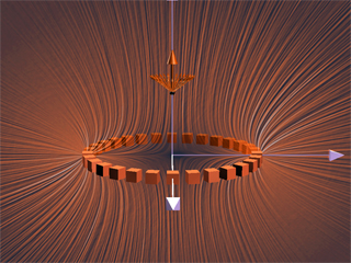
Figure 29: The electric field due to 30 charges arranged in a ring at a given observation point. The position of the observation point can be varied to see how the electric field of the individual charges adds up to give the total field.
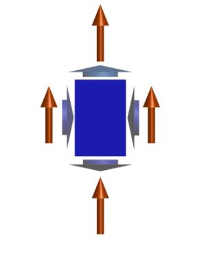
Figure 30: An imaginary box in an electric field (orange vectors). The short vectors indicate the directions of stresses transmitted by the field, either pressures (on the left or right faces of the box) or tensions (on the top and bottom faces of the box).
We now introduce the concept of stresses transmitted by fields. We will return to this concept many times. In Figure 30, we show an imaginary closed surface (an imaginary box) sitting in an electric field. If we look at the face on the left side of this imaginary box, the field on that face is perpendicular to the outwardly pointing normal to that face, and Faraday would have said that the field on that face transmits a pressure perpendicular to itself. In this case, this is a push to the right. Similarly, if we look at the face on the right side of this imaginary box, the field on that face is perpendicular to the outwardly pointing normal to that face, and Faraday would again have said that the field on that face transmits a pressure perpendicular to itself. In this case, this is a push to the left.
If we want to know the total electromagnetic force transmitted to the interior of this imaginary box in the left-right direction, we add these two transmitted stresses up. If the electric or magnetic field is homogeneous, this total electromagnetic force transmitted to the interior of the box in the left-right direction is a push to the left and an equal but opposite push to the right, and the transmitted force adds up to zero.
Similarly, if we look at the top face of the imaginary box in Figure 30, the field on that face is parallel to the outwardly pointing normal to that face, and Faraday would have said that the field on that face transmits a tension along itself across that face. In this case, this is an upward pull, just as if we had attached a string under tension to that face, pulling upward. Similarly, if we look at the bottom face of this imaginary box, the field on that face is anti-parallel to the outwardly pointing normal to that face, and Faraday would again have said that the field on that face transmits a tension along itself. In this case, this is a downward pull, just as if we had attached a string to that face, pulling downward. Note that this is a pull parallel to the outwardly pointing surface normal, whether the field is into the surface or out of the surface, since the pressures or tensions are proportional to the squares of the field magnitudes.
If we want to know the total electromagnetic force transmitted to the interior of this imaginary box in the up-down direction, we add these two transmitted stresses up. If the electric or magnetic field is homogeneous, this total electromagnetic force transmitted to the interior of the box in the up-down direction is a pull upward plus an equal and opposite pull downward, and adds up to zero.
In contrast, if the bottom face of this imaginary box is sitting inside a capacitor for which the electric field is vertical and constant, and the top face is sitting outside of that capacitor, where the electric field is zero, then there is a net pull downward, and we say that the electric field exerts a tension on the top plate of the capacitor pulling it downward. The electric field will also exert a tension on the bottom plate of the capacitor, pulling that plate upward. We can deduce this by simply looking at the electric field topology. At sufficiently high electric field, such forces will cause the capacitor plates to collapse toward one another.
The magnitude of these pressures and tensions on the various faces
of the imaginary surface in Figure 30 is given by ![]() for
the electric field. This quantity has units of force per unit
area, or pressure. It is also the energy density stored in the
electric field. Note that energy per unit volume has the same
units as pressure.
for
the electric field. This quantity has units of force per unit
area, or pressure. It is also the energy density stored in the
electric field. Note that energy per unit volume has the same
units as pressure.
Pressures and Tensions Transmitted By Electric Fields
Electromagnetic fields are mediators of the interactions between material objects. The fields transmit stresses through space. An electric field transmits a tension along itself and a pressure perpendicular to itself. The magnitude of the tension or pressure transmitted by an electric field is given by
![]() (II.5)
(II.5)
As an example of the stresses transmitted by electric fields, and
of the interchange of energy between fields and particles, consider an electric
charge with charge q > 0 moving in a constant
electric field. The charge is initially moving upward along the
negative z-axis in a constant background field ![]() .
The charge feels a constant downward force
.
The charge feels a constant downward force ![]() . The
charge eventually comes to rest at the origin, and then moves back down the
negative z-axis. This motion, and the fields that accompany it,
are shown in Figure 31, at two different times.
. The
charge eventually comes to rest at the origin, and then moves back down the
negative z-axis. This motion, and the fields that accompany it,
are shown in Figure 31, at two different times.
(a)  (b)
(b)
Figure 31: A positive charge moving in a constant electric field which points downward. (a) The total field configuration when the charge is still out of sight on the negative z-axis. (b) The total field configuration when the charge comes to rest at the origin, before it moves back down the negative z-axis.
How do we interpret the motion of the charge in terms of the stresses transmitted by the fields? Faraday would have described the downward force on the charge in Figure 31(b) as follows. In Figure 32, we show this charge surrounded by an imaginary sphere centered on it. The field lines piercing the lower half of the sphere transmit a tension that is parallel to the field. This is a stress pulling downward on the charge from below. The field lines draped over the top of the imaginary sphere transmit a pressure perpendicular to themselves. This is a stress pushing down on the charge from above. The total effect of these stresses is a net downward force on the charge.
Figure 32: An electric charge in a constant downward electric field. We surround the charge by an imaginary sphere in order to discuss the stresses transmitted across the surface of that sphere by the electric field.
Viewing the animation of Figure 31 greatly enhances Faraday’s interpretation of the stresses in the static image. As the charge moves upward, it is apparent in the animation that the electric field lines are generally compressed above the charge and stretched below the charge. This field configuration enables the transmission of a downward force to the moving charge we can see as well as an upward force to the charges that produce the constant field, which we cannot see. The overall appearance of the upward motion of the charge through the electric field is that of a point being forced into a resisting medium, with stresses arising in that medium as a result of that encroachment.
The kinetic energy of the upwardly moving charge is decreasing as more and more energy is stored in the compressed electrostatic field, and conversely when the charge is moving downward. Moreover, because the field line motion in the animation is in the direction of the energy flow, we can explicitly see the electromagnetic energy flow away from the charge into the surrounding field when the charge is slowing. Conversely, we see the electromagnetic energy flow back to the charge from the surrounding field when the charge is being accelerating back down the z-axis by the energy released from the field.
Finally, consider momentum conservation. The moving charge in the animation of Figure 31 completely reverses its direction of motion over the course of the animation. How do we conserve momentum in this process? Momentum is conserved because momentum in the positive z direction is transmitted from the moving charge to the charges that are generating the constant downward electric field (not shown). This is obvious from the field configuration shown in Figure 32. The field stress, which pushes downward on the charge, is accompanied by a stress pushing upward on the charges generating the constant field.
As a second example of the stresses transmitted by electric fields, consider a positive point charge sitting at rest at the origin in an external field which is constant in space but varies in time. This external field is uniform varies according to the equation
![]() (II.6)
(II.6)
Figure 33 shows two frames of an animation of the total electric field configuration for this situation. Figure 33(a) is at t = 0, when the vertical electric field is zero. Frame 33(b) is at a quarter period later, when the downward electric field is at a maximum. As in Figure 32 above, we interpret the field configuration in Figure 33(b) as indicating a net downward force on the stationary charge. The animation of Figure 33 shows dramatically the inflow of energy into the neighborhood of the charge as the external electric field grows in time, with a resulting build-up of stress that transmits a downward force to the positive charge.
(a) 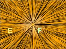 (b)
(b)

Figure 33: Two frames of an animation of the electric field around a positive charge sitting at rest in a time-changing electric field that points downward. The orange vector is the electric field and the white vector is the force on the point charge.
We can estimate the magnitude of the force on the charge in Figure 33(b) using equation (II.5) as follows. At the time shown in Figure 33(b), the distance ro above the charge at which the electric field of the charge is equal and opposite to the constant electric field is determined by the equation
![]() (II.7)
(II.7)
The surface area of a sphere of this radius is
![]() . Now
according to equation (II.5) the pressure (force per unit area) and/or tension
transmitted across the surface of this sphere surrounding the charge is of the
order of
. Now
according to equation (II.5) the pressure (force per unit area) and/or tension
transmitted across the surface of this sphere surrounding the charge is of the
order of ![]() .
Since the electric field on the surface of the sphere is of order Eo,
the total force transmitted by the field is of order
.
Since the electric field on the surface of the sphere is of order Eo,
the total force transmitted by the field is of order
![]() times
the area of the sphere, or
times
the area of the sphere, or ![]() , as
we expect.
, as
we expect.
Of course this net force is a combination of a
pressure pushing down on the top of the sphere and a tension pulling down across
the bottom of the sphere. However, the rough estimate that we
have just made demonstrates that the pressures and tensions transmitted across
the surface of this sphere surrounding the charge are plausibly of order
![]() , as
we claimed in equation (II.5).
, as
we claimed in equation (II.5).
Finally, consider two charges hanging from pendulums whose supports can be moved closer or further apart by an external agent. First, suppose the charges both have the same sign, and therefore repel. Figure 34 shows the situation when an external agent tries to move the supports (from which the two positive charges are suspended) together. The force of gravity is pulling the charges down, and the force of electrostatic repulsion is pushing them apart on the radial line joining them. The behavior of the electric fields in this situation is an example of an electrostatic pressure transmitted perpendicular to the field. That pressure tries to keep the two charges apart in this situation, as the external agent controlling the pendulum supports tries to move them together.
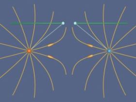
Figure 34: Two pendulums from which are suspended charges of the same sign. When we move the supports together the charges are pushed apart by the pressure transmitted perpendicular to the electric field. We artificially terminate the field lines at a fixed distance from the charges to avoid visual confusion.
In contrast, suppose the charges are of opposite signs, and therefore attract. Figure 35 shows the situation when an external agent moves the supports (from which the two positive charges are suspended) together. The force of gravity is pulling the charges down, and the force of electrostatic attraction is pulling them together on the radial line joining them. The behavior of the electric fields in this situation is an example of the tension transmitted parallel to the field. That tension tries to pull the two unlike charges together in this situation.
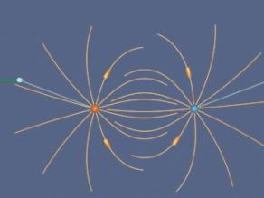
Figure 35: Two pendulums with suspended charges of opposite sign. When we move the supports together the charges are pulled together by the tension transmitted parallel to the electric field. We artificially terminate the field lines at a fixed distance from the charges to avoid visual confusion.
Electric fields are created by electric charge. If there is no electric charge present, and there never has been any electric charge present in the past, then there are no electric or magnetic fields anywhere is space. How are electromagnetic fields created and how do they come to fill up space? To explain this, consider the following scenario in which we go from the electric field being zero everywhere in space to an electric field existing everywhere in space.
Suppose we have a positive point charge sitting right on top of a negative electric charge, so that the total charge exactly cancels out. Then there is no electric field anywhere in space. Now suppose we pull these two charges apart slightly, so that there is some small distance between them, and then let them sit at that distance for a long time. There will now be a net charge, and this charge imbalance will create an electric field.
Let us see how this creation of electric field takes place in detail. Figure 36 shows three frames of an animation of the process of separating the charges. In Figure 36(a), there is no charge separation, and the electric field is zero everywhere in space. Figure 36(b) is just after the charges are first separated. We see an expanding sphere of electric fields. Figure 36(c) is a long time after the charges are separated (that is, they have been at a constant distance from another for a long time).
(a)
(b)
(c)
Figure 36: Creating an electric dipole. (a) Before any charge separation. (b) Just after the charges are separated. (c) A long time after the charges are separated.
What does this sequence tell us? It tells us first that it is electric charge that generates electric field—no charge, no field. Second, it tells us that the electric field does not appear instantaneously in space everywhere as soon as there is unbalanced charge—the electric field propagates outward from its source at some finite speed. This speed will turn out to be the speed of light. Finally, it tells us that after the charge distribution settles down and becomes stationary, so does the field configuration. The initial field pattern associated with the time dependent separation of the charge is actually a burst of “electric dipole radiation”. We return to the subject of radiation at the end of this tour. Until then, we will neglect radiation fields. The field configuration left behind after a long time is just the electric dipole pattern discussed above.
We note that the agent that pulled the charges apart had to do work to get them to separate, since as soon as they start to separate they attract each other. The agent separating them has to do work against that electric attraction. The work done by the agent goes into providing the energy carried off by radiation, as well as the energy needed to set up the final stationary electric field that we see in Figure 36c.
Finally, we ignore radiation and complete the process of separating our unlike point charges that we began in Figure 36. Figure 37 shows the complete sequence. When we finish and have moved the charges far apart, we see the characteristic radial field of a point charge.
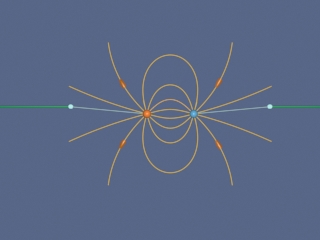
Figure 37: Creating the electric fields of two point charges by pulling apart two unlike charges initially on top of one another. We artificially terminate the field lines at a fixed distance from the charges to avoid visual confusion.
Let us look at the process of creating electric energy in a different context. We ignore energy losses due to radiation in this discussion. Figure 38 shows one frame of an animation that illustrates the following process. We start out with five negative electric charges and five positive charges, all at the same point in space. Sine there is no net charge, there is no electric field. Now we move one of the positive charges at constant velocity from its initial position to a distance L away along the horizontal axis. After doing that, we move the second positive charge in the same manner to the position where the first positive charge sits. After doing that, we continue on with the rest of the positive charges in the same manner, until all the positive charges are sitting a distance L from their initial position along the horizontal axis. Figure 38 shows the field configuration during this process. We have color coded the “grass seeds” representation to represent the strength of the electric field. Very strong fields are white, very weak fields are black, and fields of intermediate strength are yellow.
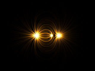
Figure 38: Creating and destroying electric energy.
Over the course of the “create” animation associated with Figure 38, the strength of the electric field grows as each positive charge is moved into place. That energy flows out from the path along which the charges move, and is being provided by the agent moving the charge against the electric field of the other charges. The work that this agent does to separate the charges against their electric attraction appears as energy in the electric field. We also have an animation of the opposite process linked to Figure 38. That is, we return in sequence each of the five positive charges to their original positions. At the end of this process we no longer have an electric field, because we no longer have an unbalanced electric charge.
Over the course of the “destroy” animation associated with Figure 38, the strength of the electric field decreases as each positive charge is returned to its original position. That energy flows from the field back to the path along which the charges move, and is now being provided to the agent moving the charge at constant speed along the electric field of the other charges. The energy provided to that agent as we destroy the electric field is exactly the amount of energy that the agent put into creating the electric field in the first place, neglecting radiative losses (such losses are small if we move the charges at speeds small compared to the speed of light). This is a totally reversible process if we neglect such losses. That is, the amount of energy the agent puts into creating the electric field is exactly returned to that agent as the field is destroyed.
There is one final point to be made. Whenever electromagnetic
energy is being created, an electric charge is moving (or being moved) against
an electric field ( ![]() ).
Whenever electromagnetic energy is being destroyed, an electric charge
is moving (or being moved) along an electric field (
).
Whenever electromagnetic energy is being destroyed, an electric charge
is moving (or being moved) along an electric field ( ![]() ).
When we return to the creation and destruction of magnetic energy, we
will find this rule holds there as well.
).
When we return to the creation and destruction of magnetic energy, we
will find this rule holds there as well.
“…As our mental eye penetrates into smaller and smaller distances and shorter and shorter times, we find nature behaving so entirely differently from what we observe in visible and palpable bodies of our surroundings that no model shaped after our large-scale experiences can ever be "true". A completely satisfactory model of this type is not only practically inaccessible, but not even thinkable. Or, to be precise, we can, of course, think of it, but however we think it, it is wrong.”
Erwin Schroedinger
The nuclear “strong” force holds protons and neutrons together, but except in unusual circumstances (e.g. atomic explosions), that force is so strong that the bonds are impossible to break, and thus the energy associated with them are essentially unavailable to us. The energies that we can easily influence in our everyday existence, and that therefore dominate the changes we see in the world about us, are electromagnetic in nature. Electromagnetic forces provide the “glue” that holds atoms together—that is, that keep electrons near protons and bind atoms together in solids. We present here a brief and very idealized (and mostly wrong) model of how that happens from a semi-classical point of view.
Figures 39 and 40 are examples of the stresses transmitted by fields, as we have seen before. In Figure 39 we have a negative charge moving past a massive positive charge and being deflected toward that charge due to the attraction that the two charges feel. This attraction is mediated by the stresses transmitted by the electromagnetic field, and the simple interpretation of the interaction shown in Figure 39 is that the attraction is primarily due to a tension transmitted by the electric fields surrounding the charges.
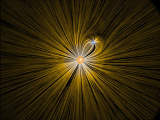
Figure 39: A negative charge moves past a massive positive particle at the origin and is deflected from its path by the stresses transmitted by the electric fields surrounding the charges.
In Figure 40 we have a positive charge moving past a massive positive charge and being deflected away from that charge due to the repulsion that the two charges feel. This repulsion is mediated by the stresses transmitted by the electromagnetic field, as we have discussed above, and the simple interpretation of the interaction shown in Figure 40 is that the repulsion is primarily due to a pressure transmitted by the electric fields surrounding the charges.
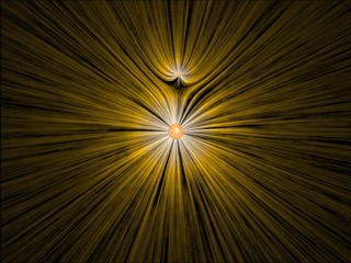
Figure 40: A positive charge moves past a massive positive particle at the origin and is deflected from its path by the stresses transmitted by the electric fields surrounding the charges.
What is the point of these two figures? The point is that there is a field or “aura” that surrounds charged objects, and the existence of this “field” is the mechanism by which they interact with other charges. The “matter” in these charges never directly “touch”. Rather, the charges interact via their fields. In what follows we will sketch how this interaction holds matter together.
Consider the interaction of four charges of equal mass shown in Figure 41. Two of the charges are positively charged and two of the charges are negatively charged, and all have the same magnitude of charge. The particles interact via the Coulomb force. We also introduce a quantum-mechanical “Pauli” force, which is always repulsive and becomes very important at small distances, but is negligible at large distances. The critical distance at which this repulsive force begins to dominate is about the radius of the spheres shown in Figure 41. This “Pauli” force is quantum mechanical in origin, and keeps the charges from collapsing into a point (i.e., it keeps a negative particle and a positive particle from sitting exactly on top of one another). Additionally, the motion of the particles is damped by a term proportional to their velocity, allowing them to "settle down" into stable (or meta-stable) states.
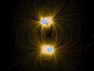
Figure 41: Four charges interacting via the Coulomb force, a repulsive Pauli force at close distances, with dynamic damping.
When these charges are allowed to evolve from the initial state, the first thing that happens (very quickly) is that the charges pair off into dipoles. This is a rapid process because the Coulomb attraction between unbalanced charges is very large. This process is called "ionic binding", and is responsible for the inter-atomic forces in ordinary table salt, NaCl. After the dipoles form, there is still an interaction between neighboring dipoles, but this is a much weaker interaction because the electric field of the dipoles falls off much faster than that of a single charge. This is because the net charge of the dipole is zero. When two opposite charges are close to one another, their electric fields “almost” cancel each other out.
Although in principle the dipole-dipole interaction can be either repulsive or attractive, in practice there is a torque that rotates the dipoles so that the dipole-dipole force is attractive. After a long time, this dipole-dipole attraction brings the two dipoles together in a bound state. The force of attraction between two dipoles is termed a “van der Waals” force, and it is responsible for intermolecular forces that bind some substances together into a solid. Note that these electrostatic forces also bind electrons to the nucleus.
Figure 42 is an interactive two-dimensional ShockWave display that shows the same dynamical situation as in Figure 41 except that we have included a number of positive and negative charges, and we have eliminated the representation of the field so that we can interact with this simulation in real time. We start the charges at rest in random positions in space, and then let them evolve according to the forces that act on them (electrostatic attraction/repulsion, Pauli repulsion at very short distances, and a dynamic drag term proportional to velocity). The particles will eventually end up in a configuration in which the net force on any given particle is essentially zero. As we saw in the animation in Figure 41 above, generally the individual particles first pair off into dipoles and then slowly combine into larger structures. Rings and straight lines are the most common configurations, but by clicking and dragging particles around, the user can coax them into more complex meta-stable formations.
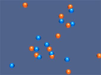
Figure 42: A two-dimensional interactive simulation of a collection of positive and negative charges affected by the Coulomb force and the “Pauli” repulsive force, with dynamic damping.
In particular, try this sequence of actions with the display. Start it and wait until the simulation has evolved to the point where you have a line of particles made up of seven or eight particles. Left click on one of the end charges of this line and drag it with the mouse. If you do this slowly enough, the entire line of chares will follow along with the charge you are virtually “touching”. When you move that charge, you are putting “energy” into the charge you have selected on one end of the line. This “energy” is going into moving that charge, but it is also being supplied to the rest of the charges via their electromagnetic fields. The “energy” that the charge on the opposite end of the line receives a little while after you start moving the first charge is delivered to it entirely by energy flowing through space in the electromagnetic field, from the site where you create that energy.
This is a microcosm of how you interact with the world. A physical object lying on the floor in front is held together by electrostatic forces. Quantum mechanics keeps it from collapsing; electrostatic forces keep it from flying apart. When you reach down and pick that object up by one end, energy is transferred from where you grasp the object to the rest of it by energy flow in the electromagnetic field. When you raise it above the floor, the “tail end” of the object never “touches” the point where you grasp it. All of the energy provided to the “tail end” of the object to move it upward against gravity is provided by energy flow via electromagnetic fields, through the complicated web of electromagnetic fields that hold the object together.
Figure 43 is an interactive three-dimensional ShockWave display that shows the same dynamical situation as in Figure 42 except that we are looking at the scene in three dimensions. This display can be rotated to view if from different angles by right-clicking and dragging in the display. We start the charges at rest in random positions in space, and then let them evolve according to the forces that act on them (electrostatic attraction/repulsion, Pauli repulsion at very short distances, and a dynamic drag term proportional to velocity). Here the configurations are more complex because of the availability of the third dimension. In particular, one can hit the “w” key to toggle a force that pushes the charges together on and off. Toggling this force on and letting the charges settle down in a “clump”, and then toggling it off to let them expand, allows the construction of complicated three dimension structures that are “meta-stable”. An example of one of these is given in Figure 43.
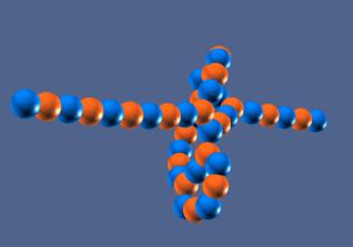
Figure 43: An three-dimensional interactive simulation of a collection of positive and negative charges affected by the Coulomb force and the “Pauli” repulsive force, with dynamic damping.
Finally, Figure 44 is an interactive ShockWave simulation that allows one to interact in two dimensions with a group of electric dipoles. The dipoles are created with random positions and orientations, with all the electric dipole vectors in the plane of the display. As we noted above, although in principle the dipole-dipole interaction can be either repulsive or attractive, in practice there is a torque that rotates the dipoles so that the dipole-dipole force is attractive. In the ShockWave simulation we see this behavior—that is, the dipoles orient themselves so as to attract, and then the attraction gathers them together into bound structures.

Figure 44: An interactive simulation of a collection of electric dipoles affected by the Coulomb force and the “Pauli” repulsive force, with dynamic damping.
Figure 45 shows an interactive simulation of a charged particle trap. Particles interact as before, but in addition each particle feels a force that pushes them toward the origin, regardless of the sign of their charge. That “trapping” force increases linearly with distance from the origin. The charges initially are randomly distributed in space, but as time increases the dynamic damping “cools” the particles and they “crystallize” into a number of highly symmetric structures, depending on the number of particles. This mimics the highly ordered structures that we see in nature (e.g., snowflakes).
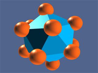
Figure 45: An interactive simulation of a particle trap. Particles interact as before, and in addition they each feel a force that pushes them toward the origin, regardless of the sign of their charge.
Here is an interesting exercise. Start the simulation. The simulation initially introduces 12 positive charges in random positions (you can of course add more particles of either sign, but for the moment we deal with only the initial 12). About half the time, the 12 charges will settle down into an equilibrium in which there is a charge in the center of a sphere on which the other 11 charges are arranged. The other half of the time all 12 particles will be arranged on the surface of a sphere, with no charge in the middle. Whichever arrangement you initially find, see if you can move one of the particles into position so that you get to the other stable configuration. To move a charge, push shift and left click, and use the arrow buttons to move it up, down, left, and right. You may have to select several different charges in turn to find one that you can move into the center, if you initial equilibrium does not have a center charge.
Here is another exercise. Put an additional 8 positive charges into the display (by pressing “p” eight times) for a total of 20 charges. By moving charges around as above, you can get two charges in inside a spherical distribution of the other 18. Is this the first number of charges for which you can get equilibrium with two charges inside? That is, can you do this with 18 charges? Note that if you push the “s” key you will get generate a surface based on the positions of the charges in the sphere, which will make its symmetries more apparent.
Finally, to connect electrostatic forces to one more example of the real world, Figure 46 is a simulation of an “electromagnetic suspension bridge”. The bridge is created by attaching a series of positive and negatively charged particles to two fixed endpoints, and adding a downward gravitational force. The tension in the "bridge" is supplied simply by the Coulomb interaction of its constituent parts and the Pauli force keeps the charges from collapsing in on each other. Initially, the bridge only sags slightly under the weight of gravity. However the user can introduce additional “neutral” particles (by pressing “o”) to stress the bridge more, until the electrostatic bonds “break” under the stress and the bridge collapses.
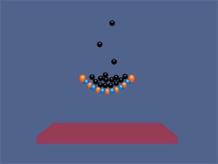
Figure 46: An interactive ShockWave simulation of an electrostatic suspension bridge.
We now turn to the nature of magnetic fields. The sequence here will be very different from the one we used for electrostatics. In electrostatics, we first introduced the electrostatic force between two charges, and then deduced from that law the nature of the electric field of a single charge. If we were going to proceed in magnetostatics in an analogous fashion, we would first introduce the force between two current-carrying segments of wire, and then deduce from that law the magnetic field of a single segment of current-carrying wire. Ampere in fact was the first to write down such an expression, and it will be implicit in what we do below, but in practice this formula is never mentioned down in introductory (or advanced!) treatments of electromagnetism.
What we do here is to put the magnetic field in its central place as the mediator of the magnetic interaction, from the outset. We first introduce the magnetic field of a single moving electric charge, and of a current-carrying wire segment, without any reference to force. We will then discuss the magnetic fields of collections of moving charges and of finite wire segments. Finally, we turn to the question of the magnetic force on a moving charge in an external magnetic field, and of a current-carrying wire segment in an external field. We never discuss directly the magnetic force between two moving charges or current-carrying wire segments without reference to the magnetic field that mediates that interaction.
The basic law that corresponds to equation (II.3) for electrostatics is the Biot-Savart Law for the magnetic field of a point electric charge moving at a velocity v. This law can be stated as
The Magnetic Field Of A Moving Point Charge
![]() (IV.1)
(IV.1)
where q is the electric charge, r is the distance between
the charge and the observation point at which the field is being measured,
the unit vector ![]() points from
the source of the field (the charge) to the observation point, and
v is the velocity of the charge. We refer readers who are not familiar
with the concept of the cross product of two vectors to an interactive ShockWave
display that illustrates the features of this operation.
points from
the source of the field (the charge) to the observation point, and
v is the velocity of the charge. We refer readers who are not familiar
with the concept of the cross product of two vectors to an interactive ShockWave
display that illustrates the features of this operation.
Figure 47 and 48 shows one frame of the animations of the magnetic field of a moving positive and negative point charge, assuming the speed of the charge is small compared to the speed of light.
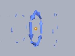
Figure 47: The magnetic field of a moving positive charge when the speed of the charge is small compared to the speed of light.
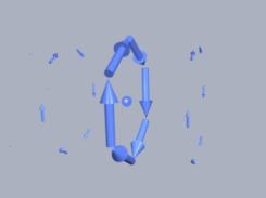
Figure 48: The magnetic field of a moving negative charge when the speed of the charge is small compared to the speed of light.
A closely related concept is the magnetic field of a current element. Suppose we have an infinitesimal current element in the form of a cylinder of cross-sectional area dA and length dl, consisting of n charge carriers per unit volume, all moving at a common velocity v along the axis of the cylinder. Let I be the current in the element, which we define as the amount of charge passing through any cross-section of the cylinder per unit time. Then I is related to the quantities introduced above by the equation
![]() (IV.2)
(IV.2)
The total number of charge carriers in the current element is just
![]() , so that
using (IV.1) and (IV.2), we have for the field dB due to these dN
charge carriers
, so that
using (IV.1) and (IV.2), we have for the field dB due to these dN
charge carriers
![]() (IV.3)
(IV.3)
If we define the vector dl to be parallel to the velocity of the charge carriers, and use (IV.1), then we can write (IV.3) as
![]() (IV.4)
(IV.4)
This is the Biot-Savart Law for the magnetic field of the current element.
Figure 49 is an interactive ShockWave display that shows the magnetic field of a current element from equation (IV.4). This interactive display allows you to move the position of the observer about the source current element to see how moving that position changes the value of the magnetic field at the position of the observer.
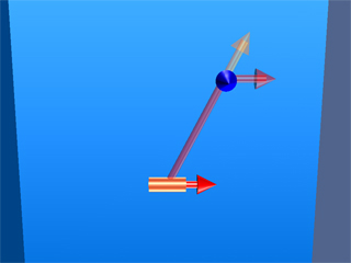
Figure 49: The magnetic field of a current element.
For a collection of point charges, we simply sum up the fields due to each of the charges. This is the Principle of Superposition.
The Magnetic Field Of A Collection Of Moving Point Charges
Consider a collection of point charges ![]() for i = 1 to
N. Let the ith charge be located in space at
for i = 1 to
N. Let the ith charge be located in space at ![]() and have velocity
and have velocity
![]() . Then the
magnetic field at a point
. Then the
magnetic field at a point ![]() is given by
is given by
 (IV.5)
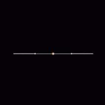
Suppose we want to calculate the magnetic fields of a number of charges moving on the circumference of a circle with equal spacing between the charges. To calculate this field we have to add up vectorially the magnetic fields of each of charges using equation (IV.5). Figure 50 shows one frame of the animation when the number of moving charges is four. Other animations show the same situation for 1, 2, and 8 charges. When we get to eight charges, a characteristic pattern emerges--the magnetic dipole pattern. Far from the ring, the shape of the field lines is the same as the shape of the field lines for an electric dipole.
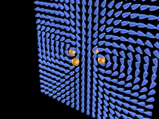
Figure 50: The magnetic field of four charges moving in a circle. We show the magnetic field vector directions in only one plane. The “bullet” like icons indicate the direction of the magnetic field at that point in the array spanning the plane.
To extend the point we have made in the section above, Figure 51 shows a ShockWave display of the vectoral addition process for the case where we have 30 charges moving on a circle. The display in Figure 51 shows an observation point fixed on the axis of the ring. As the addition proceeds, we also show the resultant up to that point (large arrow in the display).
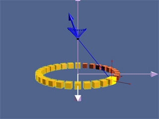
Figure 51: A ShockWave simulation of the use of the principle of superposition to find the magnetic field due to 30 moving charges moving in a circle at an observation point on the axis of the circle.
In Figure 52, we show an interactive ShockWave display that is similar to that in Figure 51, but now we can interact with the display to move the position of the observer about in space. To get a feel for the total magnetic field, we also show a “iron filings” representation of the magnetic field due to these charges. We can move the observation point about in space to see how the total field at various points arises from the individual contributions of the magnetic field of to each moving charge.
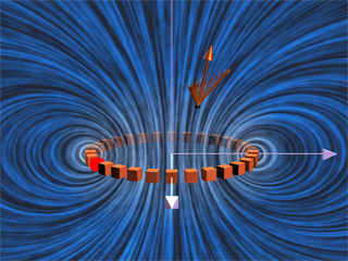
Figure 52: The magnetic field due to 30 charges moving in a circle at a given observation point. The position of the observation point can be varied to see how the magnetic field of the individual charges adds up to give the total field.
“…It appears therefore that the stress in the axis of a line of magnetic force is a tension, like that of a rope…”
J. C. Maxwell [1861].
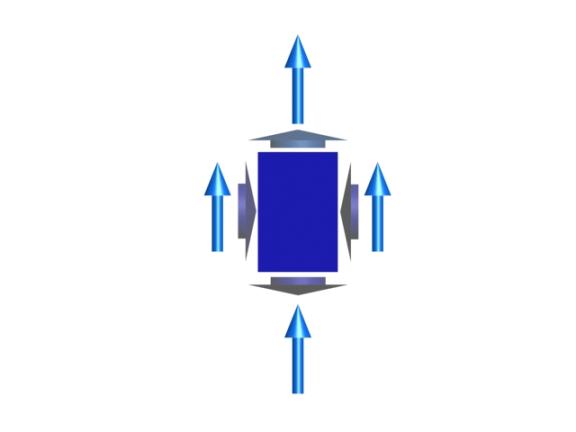
Figure 53: An imaginary box in a magnetic field (blue vectors). The short vectors indicate the directions of stresses transmitted by the field, either pressures (on the left or right faces of the box) or tensions (on the top and bottom faces of the box).
We now introduce the concept of stresses transmitted by fields. We will return to this concept many times. In Figure 53, we show an imaginary closed surface (an imaginary box) sitting in a magnetic field. If we look at the face on the left side of this imaginary box, the field on that face is perpendicular to the outwardly pointing normal to that face, and Faraday would have said that the field on that face transmits a pressure perpendicular to itself. In this case, this is a push to the right. Similarly, if we look at the face on the right side of this imaginary box, the field on that face is perpendicular to the outwardly pointing normal to that face, and Faraday would again have said that the field on that face transmits a pressure perpendicular to itself. In this case, this is a push to the left.
If we want to know the total electromagnetic force transmitted to the interior of this imaginary box in the left-right direction, we add these two transmitted stresses up. If the electric or magnetic field is homogeneous, this total electromagnetic force transmitted to the interior of the box in the left-right direction is a push to the left and an equal but opposite push to the right, and the transmitted force adds up to zero.
In contrast, if the right side of this imaginary box is sitting inside a long vertical solenoid, for which the magnetic field is vertical and constant, and the left side is sitting outside of that solenoid, where the magnetic field is zero, then there is a net push to the left, and we say that the magnetic field exerts a outward pressure on the walls of the solenoid. We can deduce this by simply looking at the magnetic field topology. At sufficiently high magnetic field, such forces will cause the walls of a solenoid to explode outward.
Similarly, if we look at the top face of the imaginary box in Figure 53, the field on that face is parallel to the outwardly pointing normal to that face, and Faraday would have said that the field on that face transmits a tension along itself across that face. In this case, this is an upward pull, just as if we had attached a string under tension to that face, pulling upward. Similarly, if we look at the bottom face of this imaginary box, the field on that face is anti-parallel to the outwardly pointing normal to that face, and Faraday would again have said that the field on that face transmits a tension along itself. In this case, this is a downward pull, just as if we had attached a string to that face, pulling downward. Note that this is a pull parallel to the outwardly pointing surface normal, whether the field is into the surface or out of the surface, since the pressures or tensions are proportional to the squares of the field magnitudes.
If we want to know the total electromagnetic force transmitted to the interior of this imaginary box in the up-down direction, we add these two transmitted stresses up. If the magnetic field is homogeneous, this total electromagnetic force transmitted to the interior of the box in the up-down direction is a pull upward plus an equal and opposite pull downward, and adds up to zero.
The magnitude of these pressures and tensions on the various faces of the
imaginary surface in Figure 53 is given by ![]() for the magnetic
field, where B is the magnitude of the magnetic field on a given
face. This quantity has units of force per unit area, or pressure. It
is also the energy density stored in the magnetic field. Note that energy
per unit volume has the same units as pressure.
for the magnetic
field, where B is the magnitude of the magnetic field on a given
face. This quantity has units of force per unit area, or pressure. It
is also the energy density stored in the magnetic field. Note that energy
per unit volume has the same units as pressure.
Pressures and Tensions Transmitted By Magnetic Fields
Electromagnetic fields are mediators of the interactions between material objects. The fields transmit stresses through space. A magnetic field transmits a tension along itself and a pressure perpendicular to itself. The magnitude of the tension or pressure transmitted by an magnetic field is given by
![]() (IV.6)
(IV.6)
As an example of the stresses transmitted by magnetic fields, consider a moving positive point charge at the origin in a rapidly changing time-dependent external field. This external field is uniform in space but varies in time according to the equation
![]() (IV.7)
(IV.7)
We assume that the variation of this field is so rapid that the charge moves only a negligible distance in one period T. Figure 54 shows two frames of an animation of the total magnetic field configuration for this situation. Figure 54(a) is at t = 0, when the vertical magnetic field is zero, and we see only the magnetic field of the moving charge (the charge is moving out of the page, so the field circulates clockwise). Frame 54(b) is at a quarter period later, when the vertically downward magnetic field is at a maximum. To the left of the charge, where the field of the charge is in the same direction as the external magnetic field (downward), the magnetic field is enhanced. To the right of the charge, where the field of the charge is opposite that of the external magnetic field, the magnetic field is reduced (and is zero at one point to the right of the charge).
(a) 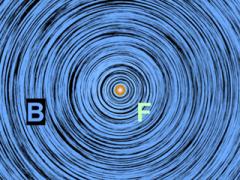 (b)
(b)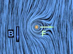
Figure 54: Two frames of an animaton of the magnetic field around a positive charge moving out of the page in a time-changing magnetic field that points downward. The blue vector is the magnetic field and the white vector is the force on the point charge.
We interpret the field configuration in Figure 54(b) as indicating a net force to the right on the moving charge. This occurs because the pressure of the magnetic field is much higher on the left as compared to the right. Note that if the charge had been moving into the page instead of out of the page, the force would have been to the left, because the magnetic pressure would have been higher on the right. The animation of Figure 54 shows dramatically the inflow of energy into the neighborhood of the charge as the external magnetic field grows, with a resulting build-up of stress that transmits a sideways force to the moving positive charge.
We can estimate the magnitude of the force on the moving charge in Figure 54(b) using equations (IV.1) and (IV.6) as follows. At the time shown in Figure 54(b), the distance ro to the right of the charge at which the magnetic field of the charge is equal and opposite to the constant magnetic field is determined by the equation
![]() (IV.8)
(IV.8)
The surface area of a sphere of this radius is
![]() . Now according
to equation (IV.6) the pressure (force per unit area) and/or tension transmitted
across the surface of this sphere surrounding the charge is of the order
of
. Now according
to equation (IV.6) the pressure (force per unit area) and/or tension transmitted
across the surface of this sphere surrounding the charge is of the order
of ![]() . Since the
magnetic field on the surface of the sphere is of order Bo,
the total force transmitted by the field is of order
. Since the
magnetic field on the surface of the sphere is of order Bo,
the total force transmitted by the field is of order ![]() times the
area of the sphere, or
times the
area of the sphere, or ![]() . Of course
this net force is a combination of a pressure pushing to the right on the
left side of the sphere and a tension pulling to the right on the right
side of the sphere. The exact expression for the force on a charge moving
in a magnetic field is
. Of course
this net force is a combination of a pressure pushing to the right on the
left side of the sphere and a tension pulling to the right on the right
side of the sphere. The exact expression for the force on a charge moving
in a magnetic field is
![]() (IV.9)
(IV.9)
The rough estimate that we have just made demonstrates
that the pressures and tensions transmitted across the surface of this sphere
surrounding the moving charge are plausibly of order ![]() . In addition,
this argument gives us some insight in to why the magnetic force on a moving
charge is transverse to the velocity of the charge and to the direction
of the background field. This is because of the side of the charge on which
the total magnetic pressure is the highest. It is this pressure that causes
the deflection of the charge.
. In addition,
this argument gives us some insight in to why the magnetic force on a moving
charge is transverse to the velocity of the charge and to the direction
of the background field. This is because of the side of the charge on which
the total magnetic pressure is the highest. It is this pressure that causes
the deflection of the charge.
To underscore the point made above, consider the trajectory of a positive charge moving in the a constant magnetic field. Figure 55 shows a charge moving toward a region where the magnetic field is vertically upward. When the charge enters the region where the external magnetic field is non-zero, it is deflected in a direction perpendicular to that field and to its velocity as it enters the field. This causes the charge to move in an arc that is a segment of a circle, until the charge exits the region where the external magnetic field in non-zero. We show in the animation the total magnetic field—that is the magnetic field of the moving charge as given by equation (IV.1), in addition to the external magnetic field. The bulging of that field on the side opposite the direction in which the particle is pushed is due to the build up in magnetic pressure on that side. It is this pressure that causes the charge to move in a circle.
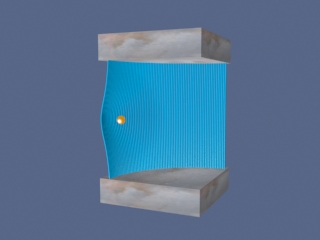
Figure 55: A charged particle moves in a magnetic field that is non-zero over the pie shaped region shown. The external field is upward.
Finally, consider momentum conservation. The moving charge in the animation of Figure 55 changes its direction of motion by ninety degrees over the course of the animation. How do we conserve momentum in this process? Momentum is conserved because momentum is transmitted by the field from the moving charge to the currents that are generating the constant external field. This is plausible given the field configuration shown in Figure 55. The magnetic field stress, which pushes the moving charge sideways, is accompanied by a tension pulling the current source in the opposite direction. To see this, look closely at the field stresses where the external field lines enter the region where the currents that produce them are hidden, and remember that the magnetic field acts as if it were exerting a tension parallel to itself. The momentum loss by the moving charge is transmitted to the hidden currents producing the constant field in this manner.
As another example of tensions and pressures transmitted by magnetic fields, Figures 56 and 57 show parallel wires carrying current in the same and in opposite directions. In the first case, the magnetic field configuration is such as to produce an attraction between the wires. In the second case the magnetic field configuration is such as to produce a repulsion between the wires.
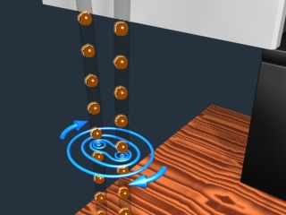
Figure 56: A visualization of the attraction of two wires carrying current in the same direction. The direction of motion of the orange spheres in the visualization indicates the direction of positive current flow.
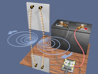
Figure 57: A visualization of the repulsion of two wires carrying current in opposite directions. The direction of motion of the orange spheres in the visualization indicates the direction of positive current flow.
As another example of tensions and pressures transmitted by magnetic fields, Figures 58 and 59 show two co-axial current-carrying circular wire loops carrying current in the same and in opposite senses. In this animation, the top loop has only 1/2 the current as the bottom loop. In the first case, the magnetic field configuration is such as to produce an attraction between the loops. In the second case the magnetic field configuration is such as to produce repulsion between the loops.
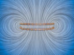
Figure 58: Two co-axial wire loops carrying current in the same sense. The loops are attracted. We show the field configuration here using the “iron filings” representation. The bottom wire loop carries twice the amount of current as the top wire loop.
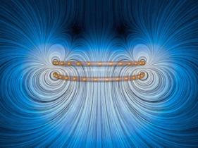
Figure 59: Two co-axial wire loops carrying current in opposite senses. The loops are repelled. We show the field configuration here using the “iron filings” representation. The bottom wire loop carries twice the amount of current as the top wire loop.
In this same vein, Figure 60 shows the force of repulsion between the magnetic field of a permanent magnet and the field of a current-carrying ring in the TeachSpin ™ Magnetic Force apparatus. The magnet is forced to have its North magnetic pole pointing downward, and the current in the top coil of the Magnetic Force apparatus is moving clockwise as seen from above. The net result is a repulsion of the magnet when the current in this direction is increased. The visualization shows the stresses transmitted by the fields to the magnet when the current in the upper coil is increased.
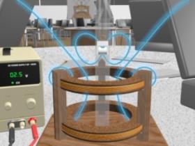
Figure 60: A magnet in the TeachSpin ™ Magnetic Force apparatus when the current in the top coil is counterclockwise as seen from the top and the North pole of the magnet is forced to point downward.
“…To understand this point, we have to consider that a [compass] needle vibrates by gathering upon itself, because of it magnetic condition and polarity, a certain amount of the lines of force, which would otherwise traverse the space about it…”
Michael Faraday [1855]
Finally, we consider a magnetic dipole in a constant background field. Historically, we note that Faraday understood the oscillations of a compass needle in exactly the way we describe here. We show in Figure 61 a magnetic dipole in a “dip needle” oscillating in the magnetic field of the earth, at a latitude approximately the same as that of Boston. The magnetic field of the earth is predominantly downward and northward at these Northern latitudes, as the visualization indicates.
To explain what is going on in this visualization, suppose that the magnetic dipole vector is initially along the direction of the earth’s field and rotating clockwise. As the dipole rotates, the magnetic field lines are compressed and stretched. The tensions and pressures associated with this field line stretching and compression results in an electromagnetic torque on the dipole that slows its clockwise rotation. Eventually the dipole comes to rest. But the counterclockwise torque still exists, and the dipole then starts to rotate counterclockwise, passing back through being parallel to the earth’s field again (where the torque goes to zero), and overshooting.
As the dipole continues to rotate counterclockwise, the magnetic field lines are now compressed and stretched in the opposite sense. The electromagnetic torque has reversed sign, now slowing the dipole in its counterclockwise rotation. Eventually the dipole will come to rest, start rotating clockwise once more, and pass back through being parallel to the field, as in the beginning. If there is no damping in the system, this motion continues indefinitely.
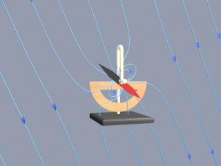
Figure 61: A magnetic dipole in the form of a dip needle rotates oscillates in the magnetic field of the earth.
What about the conservation of angular momentum in this situation? Figure 62 shows a global picture of the field lines of the dip needle and the field lines of the earth, which are generated deep in the core of the earth. If you examine the stresses transmitted between the earth and the dip needle in this visualization, you can convince yourself that any clockwise torque on the dip needle is accompanied by a counterclockwise torque on the currents producing the earth’s magnetic field. Angular momentum is conserved by the exchange of equal and opposite amounts of angular momentum between the compass and the currents in the earth’s core.
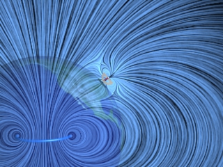
Figure
62: A magnetic dipole in the form
of a dip needle rotates oscillates in the magnetic field of the earth. We show
the currents that produce the earth’s field in this visualization.
Up to this point, the electric fields we have seen have been curl free—that is, they have the “starburst” character of the fields in Figures 6 through 8. We now consider situations in which there is a time-changing magnetic field present. Such magnetic fields are always associated with electric fields that “circulate”—that is, they have the “halo” character of the fields in Figures 11 through 13. We can determine electric fields of this nature given time changing magnetic fields by using Faraday’s Law, i.e.
![]() (V.1)
(V.1)
We now consider the process involved in creating magnetic energy. Figure 63 shows the process by which an external agent(s) creates magnetic energy. Suppose we have five rings that have a carry a number of free positive charges that are not moving. Since there is no current, there is no magnetic field. Now suppose a set of external agents come along (one for each charge) and simultaneously spin up the charges counterclockwise as seen from above, at the same time and at the same rate, in a manner that has been pre-arranged. Once the charges on the rings start to accelerate, there is a magnetic field in the space between the rings, mostly parallel to their common axis, which is stronger inside the rings than outside. This is the solenoid configuration.
As the magnetic flux through the rings grows, equation (V.1) tells us that there is an electric field induced by the time-changing magnetic field that is circulating clockwise as seen from above. The force on the charges due to this electric field is thus opposite the direction the external agents are trying to spin the rings up (counterclockwise), and thus the agents have to do additional work to spin up the charges because of their charge. This is the source of the energy that is appearing in the magnetic field between the rings—the work done by the agents against the “back emf”.
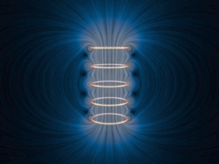
Figure 63: Creating and destroying magnetic field energy.
Over the course of the “create” animation associated with Figure 63, the agents moving the charges to a higher speed against the induced electric field are continually doing work. The electromagnetic energy that they are creating at the place where they are doing work (the path along which the charges move) flows both inward and outward. The direction of the flow of this energy is shown by the animated texture patterns in Figure 63. This is the electromagnetic energy flow that increases the strength of the magnetic field in the space between the rings as each positive charge is accelerated to a higher and higher velocity. When the external agents have gotten up the charges to a pre-determined speed, they stop the acceleration. The charges then move at a constant speed, with a constant field inside the solenoid, and zero “induced” electric field, in accordance with equation (V.1).
We also have an animation of the “destroy” process linked to Figure 63. This process proceeds as follows. Our set of external agents now simultaneously start to spin down the moving charges (which are still moving counterclockwise as seen from above), at the same time and at the same rate, in a manner that has been pre-arranged. Once the charges on the rings start to decelerate, the magnetic field in the space between the rings starts to decrease in magnitude. As the magnetic flux through the rings decreases, equation (V.1) tells us that there is now an electric field induced by the time-changing magnetic field that is circulating counterclockwise as seen from above. The force on the charges due to this electric field is thus in the same direction as the motion of the charges. In this situation the agents have work done on them as they try to spin the charges down.
Over the course of the “destroy” animation associated with Figure 63, the strength of the magnetic field decreases, and this energy flows from the field back to the path along which the charges move, and is now being provided to the agents trying to spin down the moving charges. The energy provided to those agents as they destroy the magnetic field is exactly the amount of energy that they put into creating the magnetic field in the first place, neglecting radiative losses (such losses are small if we move the charges at speeds small compared to the speed of light). This is a totally reversible process if we neglect such losses. That is, the amount of energy the agents put into creating the magnetic field is exactly returned to the agents as the field is destroyed.
There is one final point to be made. Whenever electromagnetic energy is
being created, an electric charge is moving (or being moved) against an
electric field ( ![]() ). Whenever
electromagnetic energy is being destroyed, an electric charge is moving
(or being moved) along an electric field (
). Whenever
electromagnetic energy is being destroyed, an electric charge is moving
(or being moved) along an electric field ( ![]() ). This is
the same rule we saw above when we were creating and destroying electric
energy above.
). This is
the same rule we saw above when we were creating and destroying electric
energy above.
In the example of Faraday’s Law that we gave above, the sense of the electric field associated with a time-changing magnetic field was always such as to try to resist change. We consider another example of Faraday’s Law that illustrates this same tendency in a different way. In Figure 64, we show a permanent magnet that is fixed at the origin with its dipole moment pointing upward. On the z-axis above the magnet, we have a co-axial, conducting, non-magnetic ring with radius a, inductance L, and resistance R. The center of the conducting ring is constrained to move along the vertical axis. The ring is released from rest and falls under gravity toward the stationary magnet. Eddy currents arise in the ring because of the changing magnetic flux and induced electric field as the ring falls toward the magnet, and the sense of these currents is to repel the ring when it is above the magnet.
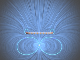
Figure 64: A perfectly conducting ring falls on the axis of a permanent magnet. The eddy currents and the resulting magnetic field stresses are such as to slow the fall of the ring. If the ring is light enough (or the magnet strong enough), the ring will levitate above the magnet.
This physical situation can be formulated mathematically in terms of three coupled ordinary differential equations for the position of the ring, its velocity, and the current in the ring. We consider in Figure 64 the particular situation where the resistance of the ring (which in our model can have any value) is identically zero, and the mass of the ring is small enough (or the field of the magnet is large enough) so that the ring levitates above the magnet. We let the ring begin at rest a distance 2a above the magnet. The ring begins to fall under gravity. When the ring reaches a distance of about a above the ring, its acceleration slows because of the increasing current in the ring. As the current increases, energy is stored in the magnetic field, and when the ring comes to rest, all of the initial gravitational potential of the ring is stored in the magnetic field. That magnetic energy is then returned to the ring as it “bounces” and returns to its original position a distance 2a above the magnet. Because there is no dissipation in the system for our particular choice of R in this example, this motion repeats indefinitely.
What are the important points to be learned from this animation? Initially, all the free energy in this situation is stored in the gravitational potential energy of the ring. As the ring begins to fall, that gravitational energy begins to appear as kinetic energy in the ring. It also begins to appear as energy stored in the magnetic field. The compressed field below the ring enables the transmission of an upward force to the moving ring as well as a downward force to the magnet. But that compression also stores energy in the magnetic field. It is plausible to argue based on the animation that the kinetic energy of the downwardly moving ring is decreasing as more and more energy is stored in the magnetostatic field, and conversely when the ring is rising. Moreover, because the field line motion is in the direction of the Poynting vector, we can explicitly see electromagnetic energy flowing away from the immediate vicinity of the ring into the surrounding field when the ring is falling and flowing back out of the surrounding field toward the immediate vicinity of the ring when it is rising.
Figure 65 shows a more realistic case in which the resistance of the ring is finite. Now energy is not conserved, and the ring eventually falls past the magnet. When it passes the magnet, the sense of the induced electric field and thus of the eddy currents reverses, and the ring is now attracted to the magnet above it, which again retards its fall.
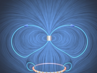
Figure 65: A ring with finite resistance falls on the axis of a magnet. We show the ring after it has fallen past the magnet, when it is attracted to the magnet above it.
There are many other examples of the falling ring and stationary magnet, or falling magnet and stationary ring, given in the animations at this link. All of them show that the effect of the electric field associated with a time-changing magnetic field is to try to keep things the same. In the limiting case of zero resistance, it can in fact achieve this goal, e.g. in Figure 64 the magnetic flux through the ring never changes over the course of the motion.
Consider an electric dipole whose dipole moment varies in time according to
![]() (VI.1)
(VI.1)
\
Figure 66 shows one frame of an animation of these fields. Close to the dipole, the field line motion and thus the Poynting vector is first outward and then inward, corresponding to energy flow outward as the quasi-static dipolar electric field energy is being built up, and energy flow inward as the quasi-static dipole electric field energy is being destroyed. Even though the energy flow direction changes sign in these regions, there is still a small time-averaged energy flow outward. This small energy flow outward represents the small amount of energy radiated away to infinity. The outer field lines detach from the dipole and move off to infinity. Outside of the point at which they neck off, the velocity of the field lines, and thus the direction of the electromagnetic energy flow, is always outward. This is the region dominated by radiation fields, which consistently carry energy outward to infinity.
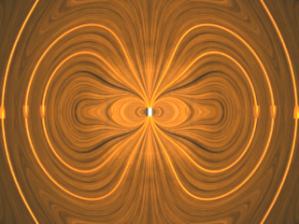
Figure 66: Electric dipole radiation from an electric dipole whose dipole moment varies by 10%.
Figure 67 shows one frame of an animation of an electric dipole whose dipole completely reverses—that is, one that has no constant term as does the dipole described by equation (VI.1).
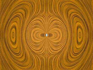
Figure 67: Electric dipole radiation from an electric dipole whose dipole moment completely reverses.
Figure 68 shows the radiation pattern at one instant of time from a quarter-wave antenna. Figure 69 shows this radiation pattern in a plane over the full period of the radiation. A quarter-wave antenna produces radiation whose wavelength is twice the tip to tip length of the antenna. This is evident in the animation of Figure 69.
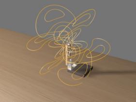
Figure 68: The azimuthal radiation pattern at one instant of time from a quarter-wave antenna.

Figure 69: The radiation pattern in one plane over the full period of a quarter-wave antenna.