Subsections
16.3 Steady-State One-Dimensional Conduction
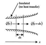
Figure 16.3:
One-dimensional heat
conduction
|
|
For one-dimensional heat conduction (temperature depending on one
variable only), we can devise a basic description of the process.
The first law in control volume form (steady flow energy equation)
with no shaft work and no mass flow reduces to the statement that
 for all surfaces
  (no heat transfer on top or
bottom of Figure 16.3). From
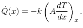
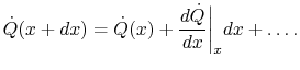
Equation (16.6), the heat transfer rate in at
the left (at
(no heat transfer on top or
bottom of Figure 16.3). From
Equation (16.6), the heat transfer rate in at
the left (at  ) is
) is
 |
(16..9) |
The heat transfer rate on the right is
 |
(16..10) |
Using the conditions on the overall heat flow and the expressions in
(16.9) and (16.10)
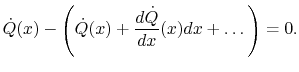 |
(16..11) |
Taking the limit as  approaches zero we obtain
 |
(16..12) |
or
 |
(16..13) |
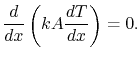
If  is constant (i.e. if the properties of the bar are
independent of temperature), this reduces to
is constant (i.e. if the properties of the bar are
independent of temperature), this reduces to
 |
(16..14) |
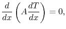
or (using the chain rule)
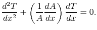 |
(16..15) |
Equation (16.14) or
(16.15) describes the temperature
field for quasi-one-dimensional steady state (no time dependence)
heat transfer. We now apply this to an example.
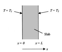
16.3.1 Example: Heat transfer through a plane slab
Figure 16.4:
Temperature boundary
conditions for a slab
|
|
For this configuration (Figure 16.4), the area
is not a function of
, i.e.
 .
Equation (16.15) thus
becomes
.
Equation (16.15) thus
becomes
 |
(16..16) |
Equation (16.16) can be integrated
immediately to yield
 |
(16..17) |
and
 |
(16..18) |
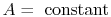
Equation (16.18) is an expression for the
temperature field where  and
and  are constants of integration.
For a second order equation, such as
(16.16), we need two boundary conditions to
determine
and
. One such set of boundary conditions can be
the specification of the temperatures at both sides of the slab as
shown in Figure 16.4, say
are constants of integration.
For a second order equation, such as
(16.16), we need two boundary conditions to
determine
and
. One such set of boundary conditions can be
the specification of the temperatures at both sides of the slab as
shown in Figure 16.4, say
 ;
;
 .
.
The condition
implies that  . The condition
 implies that
 , or
, or
 .
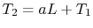
With these expressions for
and
the temperature distribution
can be written as
.
With these expressions for
and
the temperature distribution
can be written as
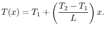 |
(16..19) |
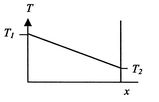
This linear variation in temperature is shown in
Figure 16.5 for a situation in which  .
.
Figure 16.5:
Temperature distribution
through a slab
|
|
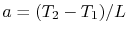
The heat flux  is also of interest. This is given by
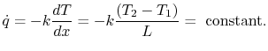 |
(16..20) |
Muddy Points
How specific do we need to be about when the one-dimensional
assumption is valid? Is it enough to say that  is small?
(MP 16.2)
is small?
(MP 16.2)
Why is the thermal conductivity of light gases such as helium
(monoatomic) or hydrogen (diatomic) much higher than heavier gases
such as argon (monoatomic) or nitrogen (diatomic)?
(MP 16.3)
UnifiedTP
|