18.2 Heat Transfer From a Fin
Fins are used in a large number of applications to increase the heat
transfer from surfaces. Typically, the fin material has a high
thermal conductivity. The fin is exposed to a flowing fluid, which
cools or heats it, with the high thermal conductivity allowing
increased heat being conducted from the wall through the fin. The
design of cooling fins is encountered in many situations and we thus
examine heat transfer in a fin as a way of defining some criteria
for design.
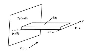
Figure 18.3:
Geometry of heat
transfer fin
|
|
A model configuration is shown in Figure 18.3. The fin is
of length  . The other parameters of the problem are indicated.
The fluid has velocity
. The other parameters of the problem are indicated.
The fluid has velocity  and temperature
  . We
assume (using the Reynolds analogy or other approach) that the heat
transfer coefficient for the fin is known and has the value
. We
assume (using the Reynolds analogy or other approach) that the heat
transfer coefficient for the fin is known and has the value  . The
end of the fin can have a different heat transfer coefficient, which
we can call
. The
end of the fin can have a different heat transfer coefficient, which
we can call  .
.
The approach taken will be quasi-one-dimensional, in that the
temperature in the fin will be assumed to be a function of  only.
This may seem a drastic simplification, and it needs some
explanation. With a fin cross-section equal to
only.
This may seem a drastic simplification, and it needs some
explanation. With a fin cross-section equal to  and a perimeter
 , the characteristic dimension in the transverse direction is
  (For a circular fin, for example,
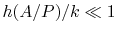
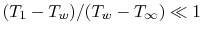
 ). The regime
of interest will be taken to be that for which the Biot number is
much less than unity,
). The regime
of interest will be taken to be that for which the Biot number is
much less than unity,
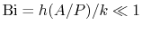 , which is a
realistic approximation in practice.
, which is a
realistic approximation in practice.
The physical content of this approximation can be seen from the
following. Heat transfer per unit area out of the fin to the fluid
is roughly of magnitude
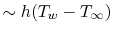 per unit area. The
heat transfer per unit area within the fin in the transverse
direction is (again in the same approximate terms)
per unit area. The
heat transfer per unit area within the fin in the transverse
direction is (again in the same approximate terms)
where  is an internal temperature. These two quantities must be
of the same magnitude. If
is an internal temperature. These two quantities must be
of the same magnitude. If
 , then
 . In other words, if
 , there is a much larger capability for heat transfer per unit
area across the fin than there is between the fin and the fluid, and
thus little variation in temperature inside the fin in the
transverse direction. To emphasize the point, consider the limiting
case of zero heat transfer to the fluid, i.e., an insulated fin.
Under these conditions, the temperature within the fin would be
uniform and equal to the wall temperature.
, there is a much larger capability for heat transfer per unit
area across the fin than there is between the fin and the fluid, and
thus little variation in temperature inside the fin in the
transverse direction. To emphasize the point, consider the limiting
case of zero heat transfer to the fluid, i.e., an insulated fin.
Under these conditions, the temperature within the fin would be
uniform and equal to the wall temperature.
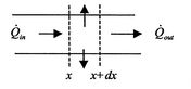
Figure 18.4:
Element of
fin showing heat transfer
|
|
If there is little variation in temperature across the
fin, an appropriate model is to say that the temperature within the
fin is a function of
only,  , and use a
quasi-one-dimensional approach. To do this, consider an element,
, and use a
quasi-one-dimensional approach. To do this, consider an element,
 , of the fin as shown in Figure 18.4. There is
heat flow of magnitude
, of the fin as shown in Figure 18.4. There is
heat flow of magnitude
 at the left-hand side
and heat flow out of magnitude
at the left-hand side
and heat flow out of magnitude
 at the right hand side. There is also heat transfer around
the perimeter on the top, bottom, and sides of the fin. From a
quasi-one-dimensional point of view, this is a situation similar to
that with internal heat sources, but here, for a cooling fin, in
each elemental slice of thickness
there is essentially a heat
sink of magnitude
at the right hand side. There is also heat transfer around
the perimeter on the top, bottom, and sides of the fin. From a
quasi-one-dimensional point of view, this is a situation similar to
that with internal heat sources, but here, for a cooling fin, in
each elemental slice of thickness
there is essentially a heat
sink of magnitude
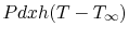 , where
  is the area
for heat transfer to the fluid.
is the area
for heat transfer to the fluid.
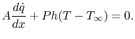
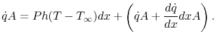
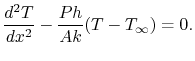
The heat balance for the element in Figure 18.4
can be written in terms of the heat flux using
 ,
for a fin of constant area:
,
for a fin of constant area:
 |
(18..7) |
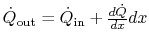
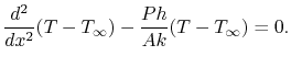
From Equation (18.7) we obtain
In terms of the temperature distribution,  :
:
 |
(18..8) |
The quantity of interest is the temperature difference
 , and we can change variables to put
Equation (18.8) in terms of this quantity
using the substitution
, and we can change variables to put
Equation (18.8) in terms of this quantity
using the substitution
Equation (18.8) can therefore be written as
 |
(18..9) |
Equation (18.9) describes the
temperature variation along the fin. It is a second order equation
and needs two boundary conditions. The first of these is that the
temperature at the end of the fin that joins the wall is equal to
the wall temperature. (Does this sound plausible? Why or why not?)
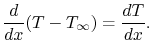
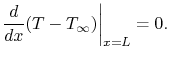
The second boundary condition is at the other end of the fin. We
will assume that the heat transfer from this end is
negligible18.1. The boundary condition at  is
is
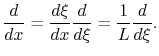
The last step is to work in terms of non-dimensional variables to
obtain a more compact description. In this we define
 as
as
 , where the
values of
range from zero to one. We also define
, where the
values of
range from zero to one. We also define
 , where
  also ranges over zero to one. The
relation between derivatives that is needed to cast the equation in
terms of
is
also ranges over zero to one. The
relation between derivatives that is needed to cast the equation in
terms of
is
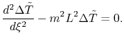
Equation (18.9) can be written
in this dimensionless form as
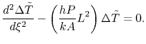 |
(18..10) |
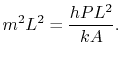
There is one non-dimensional parameter in
Equation (18.10), which we will call
 and define by
The equation for the temperature distribution we have obtained is
This second order equation has the solution
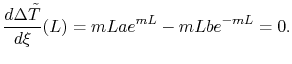
(Try it and see). The boundary condition at  is
is
The boundary condition at  is that the temperature gradient
is zero or
is that the temperature gradient
is zero or
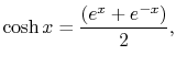
Solving the two equations given by the boundary conditions for  and
and  gives an expression for
in terms of the
hyperbolic cosine or
gives an expression for
in terms of the
hyperbolic cosine or  :
:
 |
(18..11) |
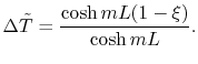
This is the solution to
Equation (18.10) for a fin with no
heat transfer at the tip. In terms of the actual heat transfer
parameters it is written as
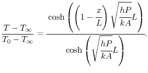 |
(18..12) |
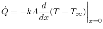
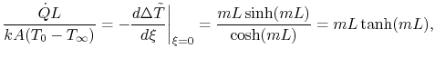
The amount of heat removed from the wall due to the fin, which is
the quantity of interest, can be found by differentiating the
temperature and evaluating the derivative at the wall,  :
:
or
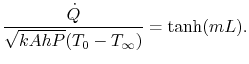 |
(18..13) |
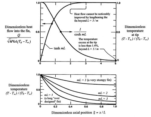
The solution is plotted in Figure 18.5,
which is taken from the book by Lienhard. Several features of the
solution should be noted. First, one does not need fins which have a
length such that
is much greater than 3. Second, the assumption
about no heat transfer at the end begins to be inappropriate as
gets smaller than 3, so for very short fins the simple expression
above would not be a good estimate. We will see below how large the
error is.
Figure 18.5:
The temperature distribution,
tip temperature, and heat flux in a straight one-dimensional fin
with the tip insulated. [From: Lienhard, A Heat Transfer
Textbook, Prentice-Hall publishers]
|
|
Muddy Points
Why did you change the variable and write the derivative  as
as
 in the equation for heat transfer in the
fin? (MP 18.2)
in the equation for heat transfer in the
fin? (MP 18.2)
What types of devices use heat transfer fins?
(MP 18.3)
Why did the Stegosaurus have cooling fins? Could the stegosaurus
have ``heating fins?'' (MP 18.4)
UnifiedTP
|