
6.302 WebLab:
Lab Client Manual
1. Introduction
1.1 The Lab Client User Interface
The Lab Client provides a platform independent Java-based user interface for running experiments at the Lab Server. It consists of a Java applet divided into two sections. The top section contains the input fields and a display of the relevant lab circuit diagram for that lab experiment. The bottom section contains the graph panels which display the Bode, Nichos and Nyquist plots for the experiment. A labelled image of the Lab Client is displayed below.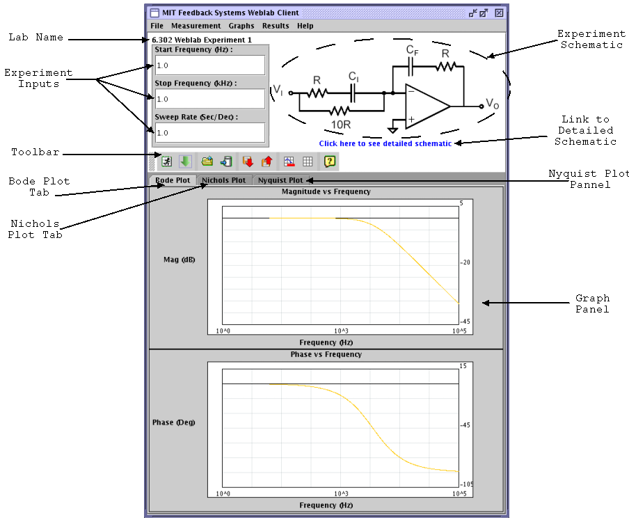
1.2 The Lab Client Toolbar
The Lab Client provides easy access to the most important functions via the toolbar. These functions are explained in further detail in the following sections. In addition, it is possible to navigate to each of these functions through the Lab Client menus.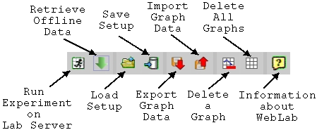
2. Starting the Lab Client
2.1 Logging into iLab
In order to log into iLab, open your browser to http://ilab.mit.edu. Input your User ID and Password in the corresponding text fields, and click the "Log In" button.2.2 Launching the Lab Client
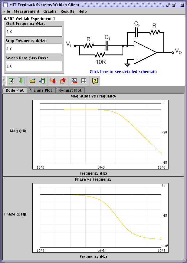
Once you have successfully logged into iLab, the Lab Client can be launched by clicking on the "Launch Client" button. The applet may then ask you to accept a certificate for authenticating the Lab Client; if this is the case, click "Yes" to accept the certificate. After the client has finished loading, you should see a window similar to the one below:
3. Running Experiments
3.1 Setting Experimental Parameters
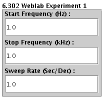
As shown below, the experimental parameters can be set by directly editing the text fields on the top left side of the applet. Each text field is labeled with the corresponding parameter name and units. These experimental parameters will then be sent to the Lab Server when submitting an experiment to be run from the Lab Client. If any of these parameters falls outside of the allowed range, a message dialog is displayed asking the user to correct the invalid experimental parameter prior to submitting the experiment.
3.2 Submitting an Experiment to the Lab Server
Once the experimental parameters have been set and they fall within the allowed range, the experiment may be submitted for execution at the Lab Server. This can be done by clicking on the leftmost icon
3.3 Canceling an Experiment Request
Once an experiment request has been submitted, an information dialog window with the queue position and estimated time until experiment completion is displayed to the user. It is then possible to cancel the experiment request by hitting the "Cancel" button on the dialog window. If the user's experiment is currently running at the Lab Server, it will not be possible to cancel the experiment at that time. Otherwise, the submitted experiment will be removed from the experiment queue at the Lab Server, and the user will be notified if their experiment request was successfully canceled.
4. Offline Data
4.1 What are Offline Data?
Offline data are similar to experimental results in that they consist of experimentally obtained data. However, offline data are not "live data" in that they are not freshly generated by running an experiment each time these data are retrieved. Offline data can be thought of as saved data for experiments that were run at some previous time by the staff, and whose results we want to make publicly available. Offline data can be manipulated at the Lab Client in exactly the same way as experimental results. These data can be exported, imported, viewed and their plots saved to a graphics file. Thus, the only difference with respect to experimental results is the manner in which these data were obtained.4.2 Retrieving Offline Data
Offline data can be retrieved by clicking on the second leftmost icon
5. Setups
5.1 What are Setups?
Setups refer to the set of experimental parameters that are specified by the user in the text fields at the Lab Client. Setups can be saved and loaded by the user both locally and remotely at the server's database.5.2 Loading Setups
A setup can be loaded by clicking on the5.3 Saving Setups
Setups can be saved by clicking on the5.4 Deleting Setups
Setups saved on the server's database can be removed by selecting "File" and "Delete Setup" from the Lab Client menu.
6. Experimental Results
6.1 Viewing Experimental Results
Experimental results can be viewed by right-clicking on the corresponding graph, and selecting "View Graph Data" from the popup menu. Alternatively, the user can select "View Graph Data" under the "Results" menu. The user will then be prompted to select the graph whose data they wish to view by selecting it from the list of available graphs. Each set of experimental results and its corresponding graph is uniquely identified by its color.
6.2 Importing Experimental Results
Experimental results can be imported by either clicking on the6.3 Exporting Experimental Results
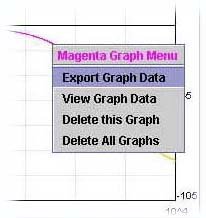
Experimental results can be exported by right-clicking on the corresponding graph, and selecting "Export Graph Data" from the popup menu, as shown below. Alternatively, the user can either click on the
6.3.1 Exporting to Matlab Format
Follow the instructions in 6.3 Exporting Experimental Results, and select "Matlab ASCII file (*.m)" from the dropdown list next to "Files of Type:".6.3.2 Exporting to CSV Format
Follow the instructions in 6.3 Exporting Experimental Results, and select "Comma-Separated Value Files (*.csv)" from the dropdown list next to "Files of Type:".
7. Managing Graphs
7.1 About the Graph Modes
There are two available graph modes:- Always Replace: this mode replaces the last set of experimental results or offline data with the newest version when running a new experiment or retrieving a new set of offline data. It is the default mode for the Lab Client.
- Always Add: this mode keeps any previously obtained sets of experimental results or offline data unless the user specifically deletes them manually. There is a fixed limit to the number of simultaneous data sets that can be managed at the Lab Client. If this limit is exceeded, the user will be asked to remove a graph data set before being able to run further experiments or retrieve additional offline data sets.
7.2 Setting the Graph Mode
The graph mode can be set at the Lab Client by opening the "Graphs" menu and selecting one of "Always Replace" or "Always Add" from the menu. The current selection will appear disabled in the menu and with a check mark.7.3 Deleting Graphs
Graphs can be deleted directly from the graph panel by right-clicking on them and selecting the "Delete this Graph" option from the popup menu. Alternatively, a graph can be removed by clicking on the7.4 Saving Graph Images
All of the plots displayed on the graph panel can be saved as a JPEG graphics file, by selecting "Save Graph Image" from the "Graphs" menu, and selecting the type of plot to save from one of Bode, Nichols and Nyquist plots. The user is then prompted to specify a file name and location where the graphics file will be stored.