A simple model of butterfly genetic mutation

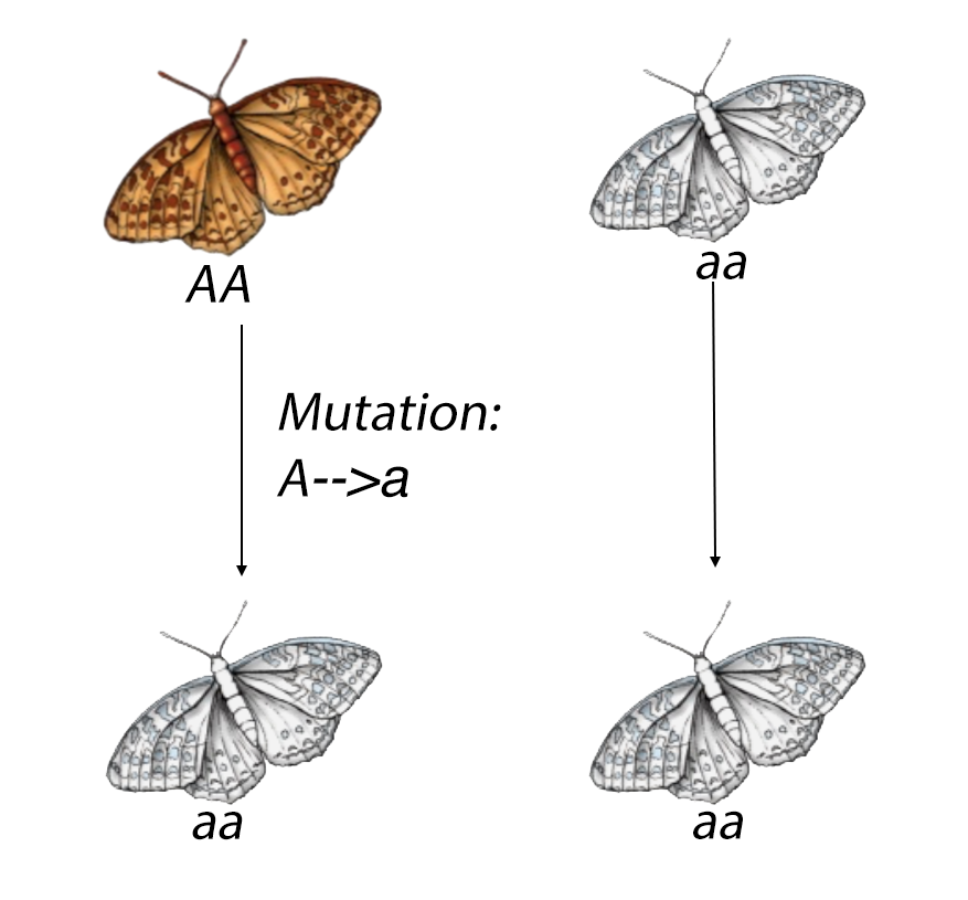
The first generation of certain butterfly has two phenomtypes, which are brown and white. Unlike the drift section, we are now allow the genetic mutaiton to happen.

Simulation

Similar to previous simulation, we define \( x_{11} \) as the number of butterflies that have \(AA \) genotype, \(x_{12}\) as the number of those have \(Aa\) and \(x_{22}\) as for \(aa\). Suppose there are \(N=x_{11}+x_{12}+x_{22}\) butterflies and we want to reproduce the next generation of \(N\) butterflies. Their parents are chosen randomly from the previous generation and randomly inherit one allel from each parent. However, \(A\) has probability \(\mu_1\) to become \(a\) and \(a\) has probability \(\mu_2\) to become \(A\) during each mating. We run this recursively to see how the ratio of each genotype evolves through \(T\) generations. Try different parameters below to see how 2 phenotypes and 3 genotypes vary.

Fixation and loss

It is not hard to find out from the simulation that it is now more difficult to eliminate one genotype. In fact it is not possible except for \(\mu_1\) and \(\mu_2\) are both zero (genetic mutation rate of human is approximately \(1.1\times 10^{-8}\) per site per generation). Imagine one gene becomes extinct in one generation, it is still possible to show up in the gene pool in the next generation due to the genetic mutation. Therefore genetic mutation is a key process for nature to keep itself being a colorful world.

Math desciption

We have mentioned the concept genotype frequency in the drift introduction page. It would be more clear if we could introduction the math description of genotype frequency and try to solve the evolution process with math symbols. We will denote a certain genotype \(i\) with its genotype frequency \(p(i)=x_i/N\). The normalized genotype frequency should be summed up to 1, that is \(\sum_i p(i)=1\). In our simulations, there are 3 genotypes denoted by \(i=11,12,22\). The interactions between 3 different genotypes are still more difficult to summarize, we then can introduce a more simplified term, allele frequency, which is the frequency of \(A\) or \(a\) in \(2N\) alleles and also well known as gene frequency.
If the population starts from a very "rare" situation, for example \(x_{11}=100,x_{12}=2,x_{22}=1\) in our simulation above, you will find that this is not going to maintain this ratio in long term in either of our two simulations. In fact, the process of proceeding to a new state can be approximated by $$\frac{\partial p_i(x,t)}{\partial t}=-\frac{\partial}{\partial x}[v(x)p_i(x,t)]+\frac{\partial^2}{\partial x^2}[D(x)p_i(x,t)],$$ where \(p_i(x,t)\) denotes the probability that \(i\)th allel occupy \(x=x_i/2N\) gene pool at time \(t\). This is called drift equation, representing a wide variaty of drift and diffusion process, including genetic drift, in which the equaion has another name of \(forward\) \(Kolmogorov\) equation. The parameters \(v(x)\) and \(D(x)\) are called drift velocity and diffusion coefficient. If you want to know more about how the equation is derived from discrete evolution to a continuous and approximately good form, the lecture notes from Prof. Mehran Kardar would be very helpful. However, we concludes some of the most interesting results of the drift equation here.

Steady probability distribution

As times goes by, the population size with the gene frequency, should be close to a steady distribution. We know that the frequency is not going to be a fixed number unless it is 0 or 1, but does change during generations. However, if we record the how often one value appears after long time simulation, we will have such a steady distribution. The steady distribution is independent of time \(\frac{\partial p^*(x)}{\partial t}=0\). We would have a equation for steady distribution from the drift equation above: $$-\frac{\partial }{\partial x}[v(x)p^*(x)]+\frac{\partial^2}{\partial x^2}[D(x)p^*(x)]=0.$$ The solution to this equation is $$p^*(x)\propto \frac{1}{D(x)}\exp{[\int^x \frac{v(x')}{D(x')}]}.$$ By taking the velocity \(v(x)=\mu_2(1-x)-\mu_1 x\) and \(D(x)=\frac{1}{4N}x(1-x)\) into the equation, we will have a nice form solution that $$p^*(x)\propto \frac{1}{x(1-x)}\times x^{4N\mu_2}\times (1-x)^{4N\mu_1}.$$ To explain the velocity and diffusion coefficient intuitively, \(v(x)\) is clearly how fast allel \(a\) mutates to \(A\) minus that part in the other direction, and diffusion process will only stop at \(x=0\) or \(1\). Details can be found in the lecture note as well.
What does this solution show? to see it more clearly, let \(\mu_1=\mu_2=\mu\), then it has a rather simple form: $$p^*(x)\propto [x(1-x)]^{4N\mu-1}.$$ Try to adjust \(N\) and \(\mu\) to see how this plot change: We can see that the population size and mutation rate together help maintaining the gene diversity. And if their product is smaller that the threshold, which is \(1/4\) in our simulation, the steady states will be attracted to the two terminals at 0 and 1. And when population size if very large, the gene frequency is always going to be centered at \(1/2\), you can also test this in the simulation above.

General mutations

In fact, mutation does not have to be constrained in existed alleles, there are also random mutations happen every seconds in every organism. Most of them occur on garbage DNA sequence, or non-coding DNA, these mutations are meaningless(or not yet to be found meaningful). A few of them occurs on critical gene sequence. Not all of them are good in terms of helping organism survive, it is believed however as the source of evolution, a few beneficial mutations survive and spread in the population. We will see this process in the next page.