Rat Behavior in Response to Reward
Changes:
A Matching-Maximizing Model
Mathew Tantama, Margaret Blayney, Dezhe Jin
9.290 Spring 2004 Midterm Project
![]()
Methods:
I. Process Characteristics
First, we can define the characteristics of the process:
|
A, B |
States |
|
TA, TB |
Stay durations |
|
lA, lB |
Reward rates of the Poisson reward baiting process |
|
pA, pB |
Leaving rates |

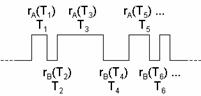
The behavior of the rat in the above process can be described as a binary signal consisting of two states A and B with consecutive stay times Ti and associated rewards ri(Ti) depicted below:
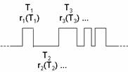
Throughout this approach we will be convention be interested in the rich side observables. We shall use the subscript A to indicate the rich side and subscript B to indicate the lean side.
II. General Algorithm
1. Approximate rat behavior by writing a stay time distribution function
2. Write a reward function in terms of experimental variables, <R> = f(TA, lA)
3. Using the empirically validated matching law to simplify the reward function
4. Maximize the reward function with respect to the rich side stay duration TA
5. Express the rich side stay duration as a function of reward rate, TA = f(lA)
III. Simple Case: Constant Frequency Behavior
As a simple case, suppose that the rat behavior results in a constant frequency signal. That is, suppose that the stay times TA and TB are constant:
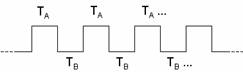
In this simplified view we can dissect the signal into repeating units of which there are two contributions to the reward received.
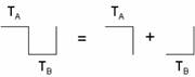
Consider the first part of the unit of which the rat is on Lever A for a stay duration TA and then switches to Lever B. The expected rewards from a stay duration TA on Lever A is lA·TA plus the reward gained from switching minus a crossover penalty “c”:
![]()
By symmetry we can similarly write the reward contribution from the second part of the unit
![]()
Thus, from one repeating unit we expect rewards of
![]()
In this simple case the repeating unit is of length TA+TB. If the total experiment is of length t then the unit occurs t·(TA+TB)-1 times. Thus, the total expected rewards is the product of the unit rewards and the number of times the unit occurs,
![]()
Now, from the data we know empirically that the matching is a reasonable approximation to make,
![]() so,
so, ![]()
Substituting,
Now, maximize <R> with respect to TA,
Simplifying,
![]()
Now, let x=Q’·lA·TA in order to see that
Thus, our model predicts that the stay duration on the rich lever is inversely proportional to the rich reward rate and proportional to the reward ratio.
IV.
Case: Behavior Approximated by a Poisson
Distribution of Stay Times
In this case we can follow an analogous approach but instead we do not have equal stay times throughout the experiment. Instead, the stay times are determined by a Poisson distribution given by the leaving rate. So, considering the behavioral signal and series of rewards received,
where we use the same reward function for Lever A and B as above
At this point we can write a function for the total expected reward rate which we will maximize.

We have simply grouped the series of rewards into those from Lever A and those from Lever B. At this point we can perform some algebraic manipulations by introducing TAtot and TBtot the total times spent on Levers A and B (not to be confused with <TA> or <TB> which are the expected average values). We also introduce Ntot the total number of events in the experiment. Then,
But we know that
![]()
And we know
So modifying our reward rate function
We know the expectation value <TA> given a Poisson probability distribution function for Lever A stay times
And we can easily evaluate the expectation value <rA> from the given integral
By symmetry, we can write our reward rate function completely as
Now we can once again use matching to simplify the reward rate function
![]()
So that our reward rate function is now
Now maximize <R’> with respect to TA
Once again we can write x=Q’·lA·TA to simplify
Thus, surprisingly even using a better approximation of the rat behavior as a Poisson process yields the same result as the simple constant frequency case. Both predict that the expected stay time on the rich side is proportional to the reward ratio and the lean side reward rate or inversely proportional to the rich side reward rate.
V. MATLAB Data Analysis
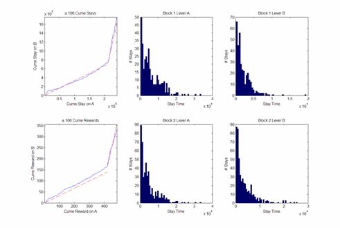
Code was written to analyze 84 data sets of rat behavior during the experiment described in the introduction and by Reference 1. Stay durations on each lever during each of the two blocks during a single trial were calculated as the time a rat first pressed a lever to the last time it released a lever before pressing the other lever. Histograms of each lever during each block were created with a standard 50 bins and analyzed for general shape. Additionally cume-cume plots were created in which the cumulative stay time on Lever A was plotted versus the cumulative stay time on Lever B for each trial. Leaving rates and reward rates were calculated as events per cumulative stay time on a given lever. Theoretical matching-only curves were plot using the set reward fraction contained in the data set. Below is an example of processed data.
Matlabe code: analyzeratdata.m