An
Example
I give here an experimental example
of a canonical heterogeneous system that helps understanding the concept
introduced earlier. It shows what are the effects of a finite tracking
depth on the mean-squared displacement distribution, and illustrates
the strength and limitations of multiple particle tracking measurements
in heterogeneous systems.
The model
system

The model system is a binary viscous
fluid. One half of the fluid is composed of water, and the other half
is composed of a 55% volume fraction solution of glycerol. Both parts
are equally represented purely viscous fluids, the water being the "fast" system
with viscosity η1 ≈
9×10⁻⁴ Pa.s and the glycerol is the "slow" fluid
with viscosity η2 ≈
9×10⁻³ Pa.s. I created such a fluid by performing two
separate experiments, one in water and one in the solution of glycerol,
both with the same concentration of probes, and I merged the results.
The tracking was performed for 30 s with 0.5 μm-diameter fluorescent
probes at a concentration of 2.9×10⁹ particles per ml.
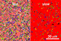
By construction none of the particle travel from one fluid to the other,
although this rare event doesn't limit the validity of our artificial
example. This canonical heterogeneous system is schematized on the figure
on the right. The same number of particle is visible in each fluid at
all time. That means that besides using the same concentration of beads
in both fluids, the same tracking parameters were also used (a detailed
discussion of this can be found in Savin & Doyle (2008), referenced here ).
This ensures that the same tracking depth is observed in both fluids,
as if the tracking was performed simultaneously on a real bimodal material.
At the end, about 180 particles were trackable at all time, 90 particles
in each fluid. Knowing that the field of view is 140 μm × 95 μm,
the tracking depth can be calculated from the known concentration and
we find it to be 4.5 μm (this method of determining the tracking depth
is very accurate, see Savin & Doyle (2008) listed here).
Also, note again that this does not mean that I have a total of 180 trajectories
at the end of the tracking. As explained in the previous section,
that would be true if the particles would remain observable the whole
duration of the movie. Here, particles are coming in and out of focus,
every time ending or beginning a new trajectory. The resulting tracking
contains a total of about 5300 trajectories, 3600 of them are obtained
in the "fast" fluid whereas 1700 are extracted from the "slow" side
of the fluid. This unbalance is a consequence of the finite depth of
tracking as explained in the previous section.
It poses some immediate problems when looking at the distribution of
msd.
).
This ensures that the same tracking depth is observed in both fluids,
as if the tracking was performed simultaneously on a real bimodal material.
At the end, about 180 particles were trackable at all time, 90 particles
in each fluid. Knowing that the field of view is 140 μm × 95 μm,
the tracking depth can be calculated from the known concentration and
we find it to be 4.5 μm (this method of determining the tracking depth
is very accurate, see Savin & Doyle (2008) listed here).
Also, note again that this does not mean that I have a total of 180 trajectories
at the end of the tracking. As explained in the previous section,
that would be true if the particles would remain observable the whole
duration of the movie. Here, particles are coming in and out of focus,
every time ending or beginning a new trajectory. The resulting tracking
contains a total of about 5300 trajectories, 3600 of them are obtained
in the "fast" fluid whereas 1700 are extracted from the "slow" side
of the fluid. This unbalance is a consequence of the finite depth of
tracking as explained in the previous section.
It poses some immediate problems when looking at the distribution of
msd.
The msd distribution
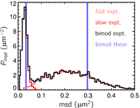
Out of these 5300 trajectories, I calculated
5300 values of msd at a lag time τ=0.1
s. I plot here the distribution of these msd. Since we know exactly the
nature of the fluid, where two different viscosities η1 and η2 are
equally represented, the distribution of viscosities in our canonical
heterogeneous fluid is known: it is two peaks at η1 and η2 of
equal heights. A correct mapping of this distribution in term of msd
should also gives us two peaks at msd1=4kTτ/(6πη1a)
and msd2=4kTτ/(6πη2a),
also of equal height (these two peaks are shown in blue on the plot on
the right-hand side). Because of the finite depth of tracking, the measured
distribution of msd is very different. First, we have much more msd calculated
from the "fast" fluid than from the "slow", as previously
explained. Second, since the msd calculated in the "fast" fluid
are mostly calculated from short trajectories, they are in general not
precisely estimated. This explains the wide spread of msd in the "fast" fluid
around their supposed value (the asymetry of the peak is a feature of
squared quantities distributions). On the other hand longer trajectories
are more frequent in the slow fluid and lead to better estimates of their
respective msd, so that the peak is sharper. In the end, the distribution
of msd calculated in the bimodal fluid is significantly deformed in two
ways: the peaks are unbalanced, and they are estimated with different
accuracies. This distribution cannot be used directly to measure mean
and variance of the msd, as we'll see in the next part.
Calculating
msd and heterogeneity
As explained in the previous section,
it is still possible to calculate unbiased estimators of the msd distribution
moments. Weighting each msd in the sample with the duration of the corresponding
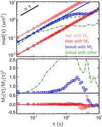
trajectories circumvents the issues presented above. In the figure on
the right I show the calculation of the ensemble mean and variance of
the msd vs. lag time using the formula of M1 and M2 given here.
Since the structure of the fluid is known, we can compare the results
with their exact expected values. The red curves correspond to the "fast" and "slow" regions
taken individually, and the blue curve is for the composite bimodal fluid.
The squares are obtained using the formula M1 and M2 of
the previous section,
and the solid lines are the expected results. For the bimodal fluid (blue
plots), we see that the formula are returning good values up until a
lag time of 0.5 s. Above this lag time, a fundamental limit of particle
tracking is reached. We explain this limit in the next part.
Notably, the estimator M1 and M2 are returning
very accurate values at τ=0.1
s, for which the distribution shown above was found.
Of interest, I also reported other possible estimates of the msd moments.
In green, the dash dotted line is the non-weighted sample mean and variance
of the msd population. As expected these estimates are failing to report
correct values. More interesting is the calculated mean msd given by
the dashed green line in the top plot: this is obtained by a weighted
sample mean where the weight is proportional to the number ni of
displacements extracted in each trajectory. This is an important quantity
because it is the one everybody uses (see the website "Particle
tracking using IDL" linked in the references).
This estimates performs well, although it is slightly biased and its
accuracy start to degrade at smaller lag times as compared to M1 (as
seen by comparing the green dashed line with the blue squares on the
top plot). This tells us that at large lag times, weighting by the displacements
number is less robust than by the duration.
Fundamental
limit
The plot above shows that significant
discrepancies are observed at large lag time, even if the mean msd is
calculated with the proper weighting. Above a certain lag time the particles
in the "fast" fluid will undergo displacements bigger then
the depth of tracking. At these large lag times, only few displacements
will be extracted from the amputated trajectories. Eventually, the displacements
calculated in the
"fast" fluid are rare and the latter will not be represented
and becomes undetectable by the multiple particle tracking measurement.
Only the "slow" fluid will be detected, and that is why the
averaged msd falls on the "slow" fluid results, as seen in
the plots of ensemble msd's mean and variance. This is a fundamental
limitation of the technique, which cannot be overcome. The assumption
of constant density only tells that as many positions are detected in
one fluid or the other. But the number of displacements can be different
from one fluid to the other because of the finite tracking depth. We
found that the detectability of a fluid can be quantified by the following
ratio that we called degree of sampling θ:
where the sum in the numerator runs only on trajectories longer than τ. This factor takes values between 0 and 1, and the limits are reached when on the one hand, no trajectory are longer than τ, thus no displacement and hence no msd can be calculated (θ=0, and the material cannot be assessed) or when all trajectory are used to calculate the msd (θ=1). As a rule of thumb, we found that in heterogeneous systems, values of M1 and M2 were unbiased for θ>80%. In the next section we
explain how to use the IDL procedures given here in
order to obtain all the information presented here, including the value
of the degree of sampling θ.
| θ(τ) = Σi:Ti>τ Ti / Σi Ti |
where the sum in the numerator runs only on trajectories longer than τ. This factor takes values between 0 and 1, and the limits are reached when on the one hand, no trajectory are longer than τ, thus no displacement and hence no msd can be calculated (θ=0, and the material cannot be assessed) or when all trajectory are used to calculate the msd (θ=1). As a rule of thumb, we found that in heterogeneous systems, values of M1 and M2 were unbiased for θ>80%. In the next section