Massachusetts Institute of Technology
Department of Urban Studies and Planning
|
11.188: Urban Planning and Social
Science Lab |
Lab Exercise 5: Vector Spatial Analysis
Out: March 9, 2020; Due: Friday, March 13, 2020, via Stellar
Overview
In this exercise you will use a few of the spatial analysis capabilities of ArcGIS to:
- Examine the location patterns of Cambridge stores by using the 'spatial join' tools to tag store location data (convenience stores, coffee shops, and pet stores) with the demographic characteristics of their neighborhood. (This is a 'point-in-polygon' operation.)
- Create an 800 meter buffer around Ames St.
- Estimate the number of children living near Ames Street by:
- Overlaying the Ames St. buffer with the Cambridge blockgroup data.
- Apportioning young children in each blockgroup that is split by the buffer, in proportion to the block group area that falls within the buffer.
- The in-lab discussion notes are here: Lab #5 notes
- The notes include some discussion of python scripts building on last Wednesday's lecture used to identify block groups falling within different cities.
Preliminaries
Launch ArcCatalog and copy the following shapefiles from the class data locker in the directory Q:\data to C:\TEMP\lab5 on a local drive:
Q:\data\camb_area_lu_1999.shp
Cambridge land use in 1999 per MassGIS (use the avl files, lu_21_1999.avl or lu37_199.avl to symbolize the layer)
Q:\data\census10\cambbgrp2010.shp
U.S. Census 2010 block groups for Cambridge. Make sure NOT to use the older 1990 cambbgrp shapefile from earlier exercises
Q:\data\census10\2010_cambtigr.shp
U.S. Census 2010 TIGER file for Cambridge from MassGIS
Q:\data\cambridge_convenience.shp
Convenience stores in Cambridge
Q:\data\cambridge_coffee.shp
Coffee shops in Cambridge
Q:\data\cambridge_pet.shp
Pet stores in Cambridge
We obtained the addresses for the features in the cambridge_convenience.shp, cambridge_coffee.shp, and cambridge_pet.shp layers from the ReferenceUSA web site on January 27, 2015. We geocoded these addresses using the free TAMU GeoServices platform. We also geocoded 4 retail locations 'manually' using GoogleMaps to obtain a higher match rate. What is geocoding and how does it work? Well, we'll be exploring address geocoding later in the semester.
Open these shapefiles in ArcMap. In order to have the ESRI and MassGIS web services available in your ArcMap session, you may wish to start by unzipping Q:\data\cambridge_shapefiles.zip into C:\temp\lab5 and then open 11.188_lab2_web.mxd. Add the new shapefiles and be sure to set the map units and display units appropriately: Since the datasets we'll be using are in Mass State Plane coordinates, select View > Data Frame Properties and in the 'General' menu bar set the map units to meters and the display units to miles. If you want, you might also change the name to something more informative than "Layers".
Part
1: Point in Polygon Spatial Join and Cluster Analyses
In this part of the lab, you will examine the demographic characteristics of the block groups in which various coffee shops are located. The point coffee shop data is contained in the shape file called cambridge_coffee.shp.
ArcMap can do 'polygons to point' overlay operations using a spatial join. We will explicitly set up a spatial join between cambridge_coffee.shp and cambbgrp2010.shp so that block group attributes can be added to the coffee shop table.
Spatial
join
- Right-Click the cambridge_coffee layer in the data frame and select joins and relates > join. The Join Data window will come up.
- Select "Join data from another layer based on spatial location" for the "What do you want to join to this layer" option.
- Choose cambbgrp2010.shp for the layer to join into the cambridge_coffee layer.
- Check the "it falls inside" option (Note that the options in the 'join data' window depend on the feature types you are trying to spatially join).
- Specify the name (coffee_bgrp.shp) of the new file and the location (your working directory) where it is stored.
- Click "OK"
The shapefile that you just created (coffee_bgrp.shp) will be added to your data frame. If you examine the attribute table for coffee_bgrp.shp you should now see the attributes of cambridge_coffee and cambbgrp2010.shp. The "Shape" columns aren't true attributes; they serve as placeholders that link to the geometry of features in the data layer in order to allow us to perform the required spatial joins.
Now we can make a thematic map of cambridge_coffee.shp using the attributes of cambbgrp2010.shp. First, you will need to join a table with the demographic data of attributes of interest to cambridge_bgrp. Let's use median household income data from the 2009-2013 American Community Survey. Join the xls file, R10905063_SL150, to coffee_bgrp. You can find the ACS table at Q:\data\Census_ACS\R10905063_SL150.xls. Can you figure out what field to base the join on? The fields that you use to join the shapefile and the xls table do not have the same name but they both contain the unique number that identifies a block group (state, county, tract, block group). Next, open the layer property window of coffee_bgrp.shp to make a "Graduated symbol" map using the field with median household income data, "ACS13_5yr_B19013001". Size the coffee shop points using the median household income of the block group that contains them. To provide additional context for interpreting these locations, create a thematic map of land use using the camb_area_lu_1999.shp layer and the lu_21_1999p.avl symbology definitions. (The 37-category symbology in lu_37_1999p.avl will also work with more detailed classification if you match it to the corresponding column in camb_area_lu_1999.shp.) Follow the same gemeral instructions as in the Mapping portion of Lab 2, except that you will use the location of coffee shops instead of housing sales. Make sure that Cambridge roads (in the TIGER file) are visible (as appropriate) to help provide context for interpreting the map.
- For the definition of the land use codes, please check the MassGIS land use code definitions in the 'datalayers' sections of the MassGIS website.
Take a close look at the pattern of coffee shops. Does anything look interesting? Write your observations as requested in the Question 1 of the assignment. Prepare a 'layout' PDF of your map and submit this as the answer for Question 2.
For extra credit, or just for fun, redo the spatial join; this time joining the 2010 block groups to the convenience store and pet store shapefiles (this requires a spatial join for each of the store layers) and display them on the map too. Do the additional store locations help you see a pattern?
Part
2: Buffer Analysis
In this part of the lab, you will analyze the demographics of the neighborhood around MIT's biological research facility on Ames Street. You will build on what you learned in the "Simple Buffering" part of Lab 3 to do a more elaborate analysis. In particular, when the buffer boundary cuts through a block group, you will apportion the attributes of that block group based on the fraction of that block group's area that lies inside the buffer. You will use ArcMap to calculate the number of children 17 years old or under who live within 800 m of the facility. (Instead of buffering a single building, we will define our 'at risk' area to be the 800 meter buffer around Ames Street as there are several biology-related buildings along Ames Street)
To begin, draw an 800 meter buffer around Ames Street. First you will select Ames Street from the 2010_cambtigr shapefile and then draw a buffer around Ames street. To do this, select the 2010_cambtigr layer, then use the Selection > Select by Attributes menu item to select the arcs where the "FULLNAME" field is "Ames St". What if we had streets for all of MA? Would we have to add to this selection query? You may have trouble spotting the arcs you just selected; use the Zoom To Selected Features button to help you find them. This feature is represented by the magnifying glass over the selection found in the toolbar at the top of your attribute table.
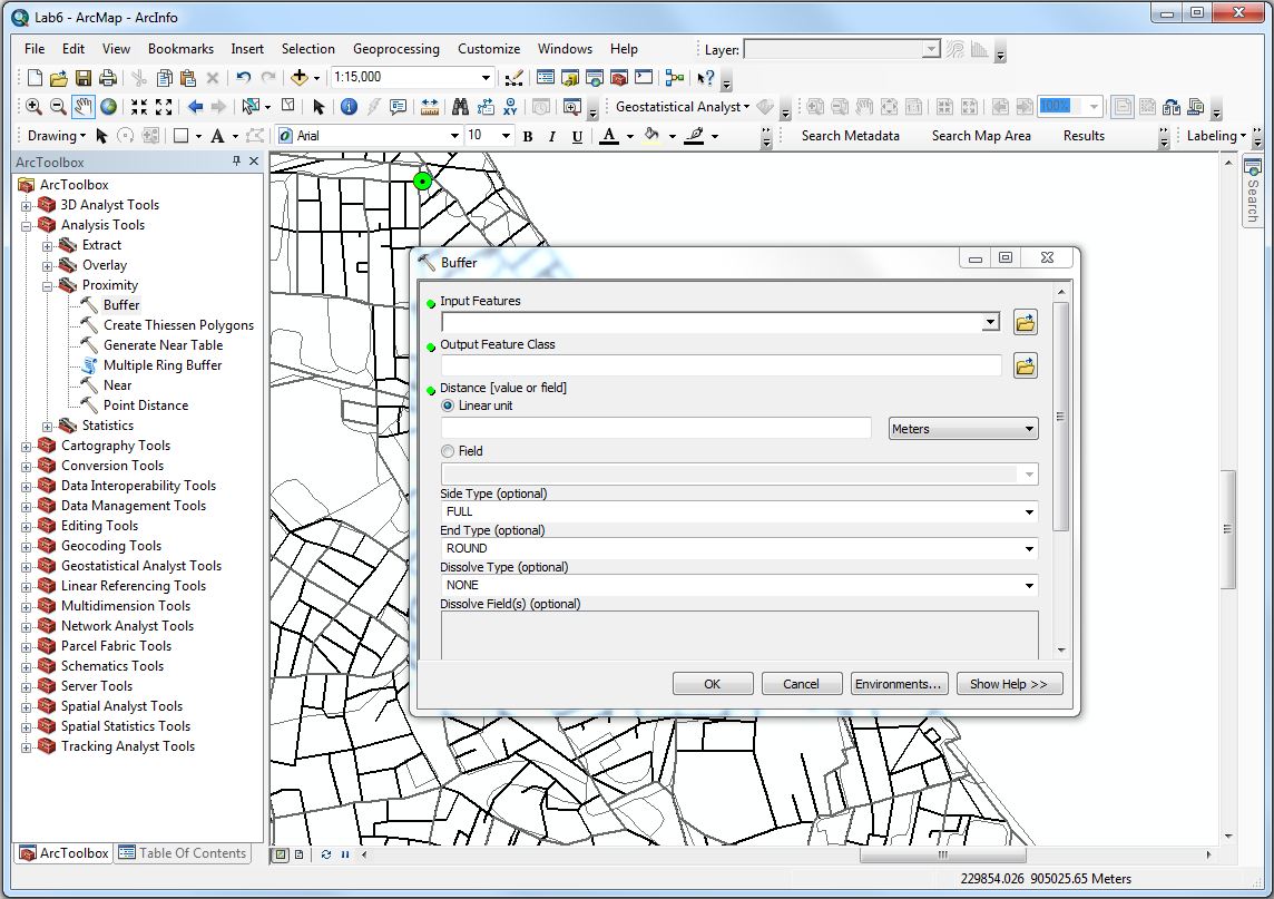
Now let's draw the 800 meter buffer around Ames Street. Use the Analysis Tools > Proximity > Buffer (see the figure below) in toolbox to start the buffer tool. First, make sure to buffer only the selected features of cambtigr. Second, specify a distance of 800 meters. In the third step, indicate you want to dissolve the barriers between the buffers by selecting "ALL" and save the results in a new layer called amesbuf in your working directory. A new data layer called amesbuf will appear in your Data Frame. Now move the amesbuf layer down so that 2010_cambtigr and the point layers display above the buffer. You should be able to clearly see the selected arcs in cambtigr at the center of the buffer.
Number of Children within 800 meters of Ames Street
Since you are interested in finding the number of children that live in the buffered area, your database must include the relevant age variables. Join the xls file, 2009_13_ACS_Age_SocialExplorerTable.xls, to cambbgrp2010. You can find this file at Q:\data\Census_ACS\2009_13_ACS_Age_SocialExplorerTable.xls. We obtained this table with selected census data for all block groups in Massachusetts from Social Explorer. Join the table to cambbgrp2010, take a look at the attribute table of cambbgrp2010.shp in ArcMap and note that there are several age-related variables that contain numeric counts:
Age Fields in the 009_13_ACS_Age_SocialExplorerTable.xls
Field
Description
SE_T007_002
Number of children under 5 years old
SE_T007_003
Number of children 5 to 9 years old
SE_T007_004
Number of children 10 to 14 years old
SE_T007_005
Number of children 15 to 17 years old
Let's take a look at the buffer relative to the block groups. Select a variable to symbolize, then adjust the display properties of the cambbgrp2010.shp layer so that only a thick black block group border is displayed: set the foreground color to transparent and the outline width to 2. Display the layer on top of both cambtigr and amesbuf. You can see that a portion of many block groups falls within the buffer area. We do not want to ignore these split block groups, nor do we want to include all their children in our count. Let's estimate the proportion of each block group that falls within the buffer? The union and intersect operations are good tools for this analysis.
Before using any of these commands let's look at the amesbuf coverage attributes created by the buffer command. When you open the buffer's attribute table, you should see that the buffer command has created a table with one row (since we only produced one buffer polygon) and three columns: the feature ID number (fid), the shape type (polygon) and a column labeled 'ld' that has a value of zero (0). (In this default case, the buffering operation will not generate a field, BufferDis, which contains the buffer distance we specified when we created the buffer).
The union and intersect operations can be used to "overlay" the block group layer with the buffer layer. The combined layer tags each feature (polygon) with attributes that indicate the original block group, and whether the polygon is inside of or outside of the buffer region.
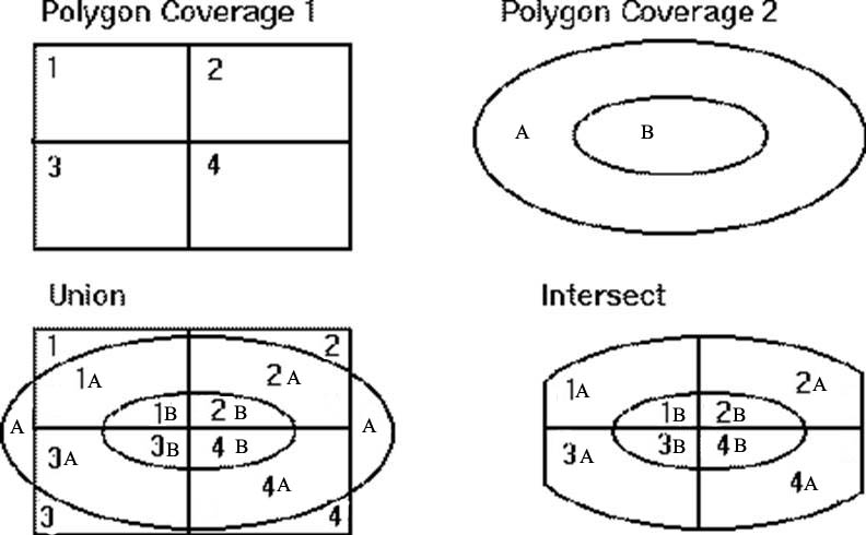
Now let's explore how the union and intersect operations differ. We will use both operations, union and intersect, to combine all the information attached to the cambbgrp2010.shp layer with the ones attached to the amesbuf coverage. The union operation computes the geometric intersection of two polygon coverages. All polygons from both coverages will be split at their intersecting pieces and preserved in the output coverage. The intersect operation, on the other hand, preserves only those features in the area common to both coverages in the output file. Visually, the difference between these two commands is:
Polygon
Overlay: Intersect
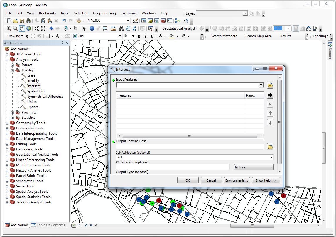
In Arctoolbox, find the intersect tool (Please see the following figure). We will use this intersect option to create a new layer, amesbgbuf_i, that combines both layers. Here is the procedure:
Procedure:
- Start up the intersect window with the Toolbox>Analysis Tool>Intersect menu item.
- Select "Input features".
- Locate cambbgrp2010.shp for "Input features".
- Locate amesbuf for the "Input features" (after this step, you will see the above two layers in the "features" portion of the tool).
- Specify the output file [your working directory]/amesbgbuf_i.shp.
- Click Finish.
The new layer, amesbgbuf_i, will appear in your view. Take a look at its attribute table. Notice that attribute columns come from both the buffer and the block group layers. There are fields named "Area" and "Perimeter" but the values are the same as in cambbgrp2010. They are the area and perimeter from the full block group polygon from which these were derived. ArcMap did not recalculate the area and perimeter for the new intersected polygons. [NOTE 1: you will also find in the amesbgbuf_i attribute table two other columns called "Shape_Area" and "Shape_Length" that are the original area and length of the buffer polygon. NOTE 2: ArcMap creates new column names in the output attribute table for amesbgbuf_i by appending the layer name plus a period in front of the original column name. That way, you can know from which original layer each column came. If the layer name (cambbgrp2010) plus the column name are too long, then ArcMap will instead rename the columns as cambbgr_1, cambbgr_2, etc. In our case, the original Area and Perimeter columns will be called "cambbgr_12" and "cambbgr_13". NOTE 3: You do not need all the original attribute columns in the output file. Consider using the 'Field" tab options to remove unneeded columns from the tables before doing the intersection.]
Open the attribute table of amesbgbuf_i, and select the Option > Add Field menu from the bottom of the amesbgbuf_i attribute table and add the following three fields to the table:
- Newarea (Type: Float)
- Arearatio (Type: Float)
- Popupto17 (Type : Float)
Click on the "Newarea" field and click the right mouse button. [At this point, you could just select 'Calculate Geometry' and compute 'Area,' without needing any python code. But we will show you how to write the python expression to get the area from the in-memory spatial object properties even if the 'calculate geometry' option were not available as a menu option.]
- Right click on your field "Newarea." Select field calculator. At the top of the box select "Python." Then set Newarea to be the python expression (including the two '!' symbols) for the 'area' parameter of the feature layer: !shape.area!
- Do you understand what the Python code is doing? The Python code gets the area value for each intersected polygon fragment in amesbgbuf_i from ArcMap's internal data structure. (The internal variable shape.area contains this area.) These values are the area within each Cambridge blockgroup that falls within the buffer. Note that these areas are less than the values in the 'Area' column for those block groups that are only partially contained within the buffer, and they should match the values in the "Shape_Area" column that ArcMap already added to the attribute table.
- You can find more about Python code in the ArcGIS help pages and on ESRI's online forum.
Now we are ready to calculate the fraction of each block group that falls within the Ames St. buffer and use that fraction to estimate the number of children living within the buffer. Assuming that the population is distributed evenly throughout each block group polygon in Cambridge, we can estimate the number of children living in the buffer by multiplying each blockgroup's children population count by the computed fraction [Newarea / Area]. (If we suspect that children are very unevenly spread across a block group, this 'uniform distribution' assumption may not be desirable.)
First, we'll calculate the ratio of the old to new area. Click on the heading for "Arearatio" and use the Calculate Values menu item again to set
Arearatio = [Newarea] / [Area]
Now we are ready to calculate our estimate of the number of children within the buffer age up to and including 17 years, adjusted for the relative portion of the block groups inside the buffer area. We are assuming that people are evenly distributed across each block group and hence the number of people falling within a buffer is proportional to the area of the polygon within the buffer area. Click on the heading for "Popupto17" and use the Calculate Values menu item again to set:
Popupto17 = ( [2009_13_15] + [2009_13_16] + [2009_13_17] + [2009_13_18]) * [Arearatio] Note: The field names changed when we did the intersect, these are different than the field names in 009_13_ACS_Age_SocialExplorerTable.xls. DOUBLE CHECK your field names before performing the calculation. The intersect will maintain the order of your variables but not the names. On our end, variable SE_T007_002 turned into F_2009__15.
At this point, stop editing the table and save your results. Now you can use the Selection > Statistics menu item to calculate the sum of the estimates across all the block groups. This sum is your estimate of the number of children 17 or younger within 1 km of the biological research facility at MIT. This is the answer to Question 3 of the lab assignment. Question 4 asks you to make a thematic map that documents your efforts.

Polygon
Overlay: Union
Now let's see how union is different from intersect. Let's do the same operation of combining both coverages and apportioning people along the buffer boundary, but this time using the union option in the Analysis Tools> Overlay. We shall call the output coverage amesbgbuf_u.
Repeat all the steps in the "Intersect" section above, with these changes:
- In the Analysis Tools, choose "Union" rather than "Intersect." Make sure you do not have any features selected.
- Make the name of the output layer amesbgbuf_u.shp instead of amesbgbuf_i.shp.
- Before you calculate the statistics on amesbgbuf_u.shp, select only those block groups that lie within the buffer. You can identify these because the "FID_amesbu" field (carried over from the buffer attribute table) contains a '0' value for these cases. (The portions of blockgroups that are outside the buffer have a '-1' value.) When you union the layers, all the attributes from both layers are carried over into the new layer. Logically, if a polygon is outside the buffer, then it is not possible to assign any fields from the buffer layer to that polygon. To compensate, ArcMap will populate these fields in these records with zeroes (for numeric fields). You will need to use the Select by Attribute menu item to restrict the rows to those within the buffer before performing the statistics calculation. If you don't, your answer will be very different than that in the "intersect" part of the exercise.
Refer to the information in the "About Union" box to help you decide what the "input" and "overlay" layers are. You should obtain the same numerical results for the child count with either the union or the intersect operation. The geography, however, will look considerably different. For your calculations to work, however, you'll need to keep track of which polygons in the amesbgbuf_u.shp layer were originally inside the buffer; these will be the polygons that have a zero value in the "FID_amesbu" field. Why is this not an issue with the layer you made with the intersect operation? Think about how union is different from intersect even though you can use either as a step toward the same end. Also pay attention to the number of features in your union file and think about which features do you want to include when running the summary option. Write your comments in the Question 5 section of the assignment.
Part
3: Other Spatial Analysis preparation tools (Optional)
-
Dissolving features and clipping layers
The above exercises only scratches the surface of spatial analysis tools in ArcGIS. We don't have time for more required exercises. This optional exercise focuses on two common operations:
- DISSOLVE - suppose we have a census block group map and we wish to create a census tract map. We can use the 'dissolve' tool to eliminate the block group boundaries that lie within a census tract.
- CLIP - this command acts like a cookie cutter.
For both these tools, appropriate handling of the feature attributes is the tricky part.
Rather than constructing a new exercise, we refer you to the "dissolve" and "clipping" exercises in the "Getting to know ArcGIS" textbook that is on reserve for the class. We have copied the data for these exercises into Q:\data\chapter11 in the class locker.
Please copy and paste all files and directories under Q:\data\chapter11 into your personal working space. In the chapter11 sub-directory, you will find two ArcGIS map document files: ex11a.mxd and ex11c.mxd. Open each document file using ArcMap and do the exercises as instructed in the text book "Getting to know ArcGIS" page 270 (ex11a) and page 282 (ex11c). You do not have to turn in any of your output from Part 3.
Assignment
Please
use the
assignment page to complete your assignment.
Back to the 11.188
Home Page. Back
to the CRN Home
Page.
Created by Raj Singh. Modified for 1999-2009 by Thomas H.
Grayson, Joseph Ferreira, Jeeseong
Chung, Jinhua Zhao, Xiongjiu Liao, and
Diao Mi,
Yang Chen, Yi Zhu, Eric Schultheis,
and Juan Camilo
Osorio.
Last modified 11 March, 2018 [jf]