|
|
|
| Thermodynamics and Propulsion | |
|
Next: 18.6 Muddiest Points on Up: 18. Generalized Conduction and Previous: 18.4 Modeling Complex Physical Contents Index
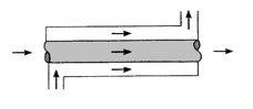
The general function of a heat exchanger is to transfer heat from
one fluid to another. The basic component of a heat exchanger can be
viewed as a tube with one fluid running through it and another fluid
flowing by on the outside. There are thus three heat transfer
operations that need to be described:
| |||||||||||||||||||||||||
|
[Finned with both
fluids unmixed.]
 [Unfinned
with one fluid mixed and the other unmixed]
[Unfinned
with one fluid mixed and the other unmixed]
|
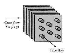
Alternatively, the fluids may be in cross flow (perpendicular to
each other), as shown by the finned and unfinned tubular heat
exchangers of Figure 18.9. The two
configurations differ according to whether the fluid moving over the
tubes is unmixed or mixed. In
Figure 18.9(a), the fluid is said to be
unmixed because the fins prevent motion in a direction (![]() ) that is
transverse to the main flow direction (
) that is
transverse to the main flow direction (![]() ). In this case the fluid
temperature varies with
). In this case the fluid
temperature varies with ![]() and
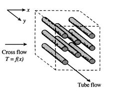
and ![]() . In contrast, for the unfinned
tube bundle of Figure 18.9(b), fluid
motion, hence mixing, in the transverse direction is possible, and
temperature variations are primarily in the main flow direction.
Since the tube flow is unmixed, both fluids are unmixed in the
finned exchanger, while one fluid is mixed and the other unmixed in
the unfinned exchanger.
. In contrast, for the unfinned
tube bundle of Figure 18.9(b), fluid
motion, hence mixing, in the transverse direction is possible, and
temperature variations are primarily in the main flow direction.
Since the tube flow is unmixed, both fluids are unmixed in the
finned exchanger, while one fluid is mixed and the other unmixed in
the unfinned exchanger.
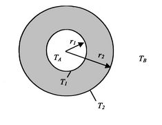
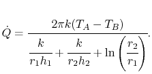
To develop the methodology for heat exchanger analysis and design, we look at the problem of heat transfer from a fluid inside a tube to another fluid outside.
We examined this problem before in Section 17.2 and found that the heat transfer rate per unit length is given by
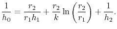
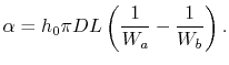
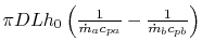
It is useful to define an overall heat transfer coefficient ![]() per unit length as
per unit length as
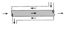
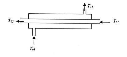
A schematic of a counterflow heat exchanger is shown in Figure 18.11. We wish to know the temperature distribution along the tube and the amount of heat transferred.
The objective is to find the mean temperature of the fluid at ![]() ,
,
![]() , in the case where fluid comes in at
, in the case where fluid comes in at ![]() with temperature
with temperature
![]() and leaves at
and leaves at ![]() with temperature
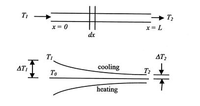
with temperature ![]() . The expected
distribution for heating and cooling are sketched in
Figure 18.12.
. The expected
distribution for heating and cooling are sketched in
Figure 18.12.
For heating (![]() ), the heat flow from the pipe wall in a
length
), the heat flow from the pipe wall in a
length ![]() is
is
where
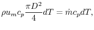
where
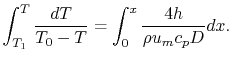
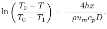
Carrying out the integration,
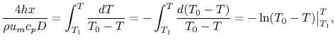
i.e.,
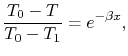
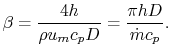
where
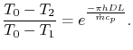
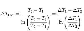
This is the temperature distribution along the pipe. The exit temperature at
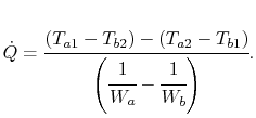
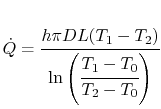
The total rate of heat transfer is therefore
 |
|
|
or
| |
| (18..27) | |
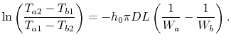
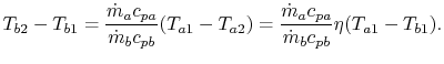
We return to our original problem, to Figure 18.11, and write an overall heat balance between the two counterflowing streams as
From a local heat balance, the heat given up by stream
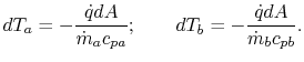
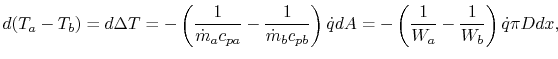
where
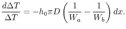
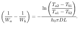
Integrating from
We know that
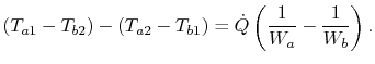
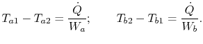
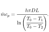
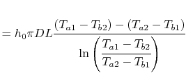
Solving for the total heat transfer:
 in terms of other
parameters as
in terms of other
parameters as
 |
(18..35) | |
|
or
| ||
| (18..36) | ||
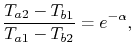
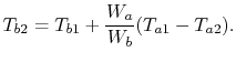
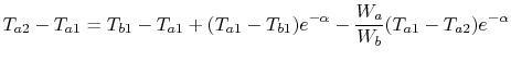
Suppose we know only the two
inlet temperatures ![]() ,
, ![]() , and we need to find the
outlet temperatures. From (18.31),
, and we need to find the
outlet temperatures. From (18.31),
|
or, rearranging,
| ||
| (18..37) | ||
or
We examine three examples.
![]() can approach zero at cold end.
can approach zero at cold end.
![]() as
as ![]() , surface area,
, surface area,
 .
.
Maximum value of ratio
![]()
Maximum value of ratio
![]() .
.
![]() is negative,
is negative,
![]() as
as
![]()
Maximum value of ratio
![]()
Maximum value of ratio
![]() .
.
![]()
temperature difference remains uniform, ![]() .
.
 [Counterflow]