|
|
|
| Thermodynamics and Propulsion | |
Subsections
[VWB&S, 6.1, 6.2]
| ||||||||||||||||||||||||||||||||||||||||||||||||||||||||||||||||||||||||||||||||||||||||||||
 |
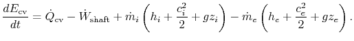
The first law of thermodynamics can be written as a rate equation:
where
 |
||
 |
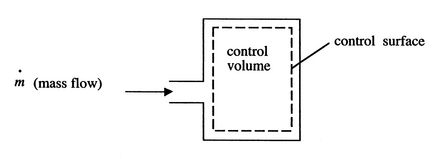
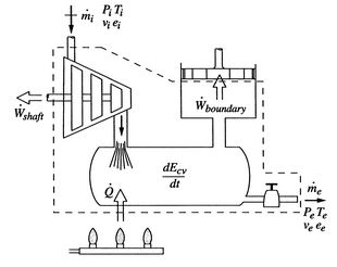
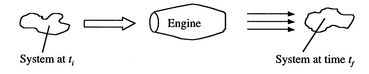
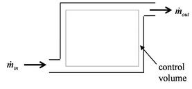
To derive the first law as a rate equation for a control volume we proceed as with the mass conservation equation. The physical idea is that any rate of change of energy in the control volume must be caused by the rates of energy flow into or out of the volume. The heat transfer and the work are already included and the only other contribution must be associated with the mass flow in and out, which carries energy with it. Figure 2.10 shows two schematics of this idea. The desired form of the equation will be
|
[Simple]
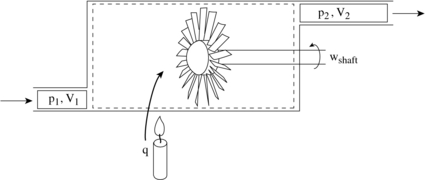 [More General]
|
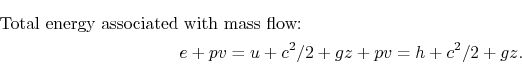
The fluid that enters or leaves has an amount of energy per unit mass given by
where
The net rate of flow work is
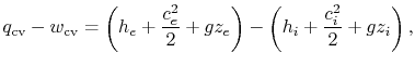
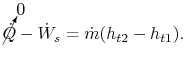
Including all possible energy flows (heat, shaft work, shear work, piston work, etc.), the first law can then be written as:

where
We can then combine the specific internal energy term, ![]() , in
, in ![]() and the specific flow work term,
and the specific flow work term, ![]() , to make the enthalpy appear:
, to make the enthalpy appear:

For most of the applications in this course, there will be no shear work and no piston work. Hence, the first law for a control volume will be most often used as:
In the special case of a steady-state flow,
 |
 |
Muddy Points
What is shaft work? (MP 2.5)
What distinguishes shaft work from other works? (MP 2.6)
Definition of a control volume (MP 2.7)
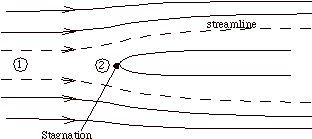
Suppose that our steady flow control volume is a set of streamlines describing the flow up to the nose of a blunt object, as in Figure 2.11.
|
The streamlines are stationary in space, so there is no external work done on the fluid as it flows. If there is also no heat transferred to the flow (adiabatic), then the steady flow energy equation becomes
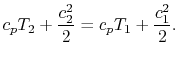 |
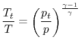
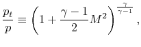
The quantity that is conserved is defined as the stagnation temperature,
 |
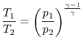
||
|
or
| ||
 |
||
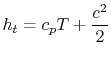
It is also convenient to define the stagnation enthalpy,
 |
 |
 |
 |
An area of common confusion is the frame dependence of stagnation quantities. The stagnation temperature and stagnation pressure are the conditions the fluid would reach if it were brought to zero speed relative to some reference frame, via a steady adiabatic process with no external work (for stagnation temperature) or a steady, adiabatic, reversible process with no external work (for stagnation pressure). Depending on the speed of the reference frame the stagnation quantities will take on different values.
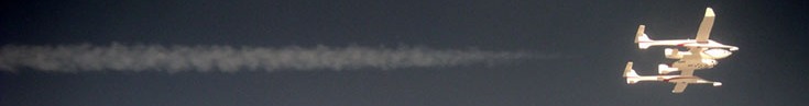
For example, consider a high speed reentry vehicle traveling through
the still atmosphere, which is at temperature, ![]() . Let's place our
reference frame on the vehicle and stagnate a fluid particle on the
nose of the vehicle (carrying it along with the vehicle and thus
essentially giving it kinetic energy). The stagnation temperature
of the air in the vehicle frame is
. Let's place our
reference frame on the vehicle and stagnate a fluid particle on the
nose of the vehicle (carrying it along with the vehicle and thus
essentially giving it kinetic energy). The stagnation temperature
of the air in the vehicle frame is
 |
The confusion comes about because ![]() is usually referred to as the
static temperature. In common language this has a similar meaning as
``stagnation,'' but in fluid mechanics and thermodynamics
static is used to label the thermodynamic properties
of the gas (
is usually referred to as the
static temperature. In common language this has a similar meaning as
``stagnation,'' but in fluid mechanics and thermodynamics
static is used to label the thermodynamic properties
of the gas (![]() ,
, ![]() , etc.), and these are not frame dependent.
, etc.), and these are not frame dependent.
Thus in our re-entry vehicle example, looking at the still atmosphere from the vehicle frame we see a stagnation temperature hotter than the atmospheric (static) temperature. If we look at the same still atmosphere from a stationary frame, the stagnation temperature is the same as the static temperature.
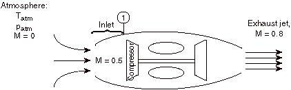
For the case shown below, a jet engine is sitting motionless on the ground prior to take-off. Air is entrained into the engine by the compressor. The inlet can be assumed to be frictionless and adiabatic.
Considering the state of the gas within the inlet, prior to passage into the compressor, as state (1), and working in the reference frame of the motionless airplane:
The stagnation temperature of the atmosphere,
![]() ,
is equal to
,
is equal to
![]() since it is moving the same speed as
the reference frame (the motionless airplane). The steady flow
energy equation tells us that if there is no heat or shaft work (the
case for our adiabatic inlet) the stagnation enthalpy (and thus
stagnation temperature for constant
since it is moving the same speed as
the reference frame (the motionless airplane). The steady flow
energy equation tells us that if there is no heat or shaft work (the
case for our adiabatic inlet) the stagnation enthalpy (and thus
stagnation temperature for constant ![]() ) remains unchanged. Thus
) remains unchanged. Thus
![]()
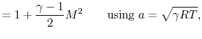
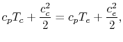
If
![]() then
then
![]() since the flow is moving at station 1 and therefore some of the
total energy is composed of kinetic energy (at the expense of
internal energy, thus lowering
since the flow is moving at station 1 and therefore some of the
total energy is composed of kinetic energy (at the expense of
internal energy, thus lowering ![]() )
)
Equal, by the same argument as 1.
Less than, by the same argument as 2.
The form of the ``Steady Flow Energy Equation'' (SFEE) that we will most commonly use is Equation 2.11 written in terms of stagnation quantities, and neglecting chemical and potential energies,
The steady flow energy equation finds much use in the analysis of power and propulsion devices and other fluid machinery. Note the prominent role of enthalpy.
Muddy Points
What is the difference between enthalpy and stagnation enthalpy? (MP 2.8)
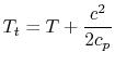
Using what we have just learned we can attack the tank filling problem solved in Section 2.3.3 from an alternate point of view using the control volume form of the first law. In this problem the shaft work is zero, and the heat transfer, kinetic energy changes, and potential energy changes are neglected. In addition there is no exit mass flow.
The control volume form of the first law is therefore

The equation of mass conservation is

Combining we have
Integrating from the initial time to the final time (the incoming enthalpy is constant) and using
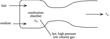
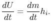
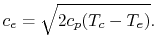
A liquid bi-propellant rocket consists of a thrust chamber and nozzle and some means for forcing the liquid propellants into the chamber where they react, converting chemical energy to thermal energy.
Once the rocket is operating we can assume that all of the
flow processes are steady, so it is appropriate to use the
steady flow energy equation. Also, for now we will assume that the
gas behaves as a perfect gas with constant specific heats, though in
general this is a poor approximation. There is no external
work, and we assume that the flow is adiabatic. We define
our control volume as going between location ![]() , in the chamber,
and location
, in the chamber,
and location ![]() , at the exit, and then write the First Law as
, at the exit, and then write the First Law as
 |
 |
 |
![$\displaystyle c_e = \sqrt{2 c_p T_c \left[1 - \left(\frac{p_e}{p_c}\right)^{\frac{\gamma-1}{\gamma}}\right]}.$](img300.png) |
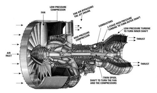
Consider for example the PW4084 pictured in Figure 2.15. The engine is designed to produce about 84,000 lbs of thrust at takeoff. The engine is a two-spool design. The fan and low pressure compressor are driven by the low pressure turbine. The high pressure compressor is driven by the high pressure turbine. We wish to find the total shaft work required to drive the compression system.
 |
 |
 |
 |
UnifiedTP
![$\displaystyle \dot{Q}_{\textrm{cv}} - \dot{W}_{\textrm{cv}} = \dot{m}\left[\left(h_e+\frac{c_e^2}{2}+gz_e\right)-\left(h_i+\frac{c_i^2}{2}+gz_i\right)\right],$](img263.png)