Subsections
[VW, S & B: 9.8-9.9, 9.12]
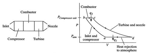
The Brayton cycle (or Joule cycle) represents the operation of a gas
turbine engine. The cycle consists of four processes, as shown in
Figure 3.13 alongside a sketch of an engine:
- a - b Adiabatic, quasi-static (or reversible)
compression in the inlet and compressor;
- b - c Constant pressure fuel combustion (idealized as constant
pressure heat addition);
- c - d Adiabatic, quasi-static (or reversible) expansion in the
turbine and exhaust nozzle, with which we
- take some work out of the air and use it to drive the compressor, and
- take the
remaining work out and use it to accelerate fluid for jet
propulsion, or to turn a generator for electrical power generation;
- d - a Cool the air at constant pressure back to its initial
condition.
Figure 3.13:
Sketch of the jet engine
components and corresponding thermodynamic states
|
|
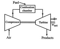
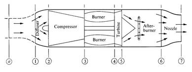
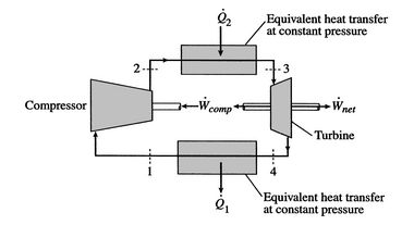
The components of a Brayton cycle device for jet propulsion are
shown in Figure 3.14. We will typically represent these
components schematically, as in
Figure 3.15. In practice, real Brayton
cycles take one of two forms. Figure 3.16(a)
shows an ``open'' cycle, where the working fluid enters and then
exits the device. This is the way a jet propulsion cycle works.
Figure 3.16(b) shows the alternative, a closed
cycle, which recirculates the working fluid. Closed cycles are used,
for example, in space power generation.
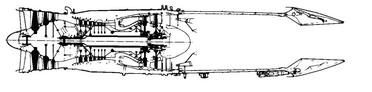
Figure 3.14:
Schematics of typical military
gas turbine engines. Top: turbojet with afterburning, bottom: GE
F404 low bypass ratio turbofan with afterburning (Hill and Peterson,
1992).
|
|
Figure 3.15:
Thermodynamic model of gas
turbine engine cycle for power generation
|
|
Figure 3.16:
Options for operating Brayton cycle gas turbine engines
[Open cycle operation]
[Closed cycle operation]

|
Muddy Points
Would it be practical to run a Brayton cycle in reverse and use it
as refrigerator? (MP 3.10)
3.7.1 Work and Efficiency
The objective now is to find the work done, the heat absorbed, and
the thermal efficiency of the cycle. Tracing the path shown around
the cycle from  -
- -
- -
- and back to
, the first law gives
(writing the equation in terms of a unit mass),
and back to
, the first law gives
(writing the equation in terms of a unit mass),
Here  is zero because
  is a function of state, and any
cycle returns the system to its starting state3.2. The net work done is therefore
is a function of state, and any
cycle returns the system to its starting state3.2. The net work done is therefore
where  ,
,  are defined as heat received by the system
(
is negative). We thus need to evaluate the heat transferred
in processes
-
and
-
.
are defined as heat received by the system
(
is negative). We thus need to evaluate the heat transferred
in processes
-
and
-
.
For a constant pressure, quasi-static process the heat exchange per
unit mass is
We can see this by writing the first law in terms of enthalpy (see
Section 2.3.4) or by remembering the
definition of  .
.
The heat exchange can be expressed in terms of enthalpy differences
between the relevant states. Treating the working fluid as a perfect
gas with constant specific heats, for the heat addition from the
combustor,
The heat rejected is, similarly,
The net work per unit mass is given by
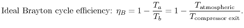
The thermal efficiency of the Brayton cycle can now be expressed in
terms of the temperatures:
 |
(3..8) |
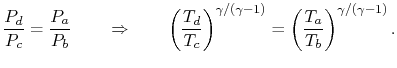
To proceed further, we need to examine the relationships between the
different temperatures. We know that points
and
are on a
constant pressure process as are points
and
, and  ;
;
 . The other two legs of the cycle are adiabatic and
reversible, so
. The other two legs of the cycle are adiabatic and
reversible, so
Therefore
 , or, finally,
 .
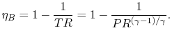
Using this relation in the expression for thermal efficiency,
Eq. (3.8) yields an expression for
the thermal efficiency of a Brayton cycle:
.
Using this relation in the expression for thermal efficiency,
Eq. (3.8) yields an expression for
the thermal efficiency of a Brayton cycle:
 |
(3..9) |
The temperature ratio across the compressor,
 . In terms
of compressor temperature ratio, and using the relation for an
adiabatic reversible process we can write the efficiency in terms of
the compressor (and cycle) pressure ratio, which is the parameter
commonly used:
. In terms
of compressor temperature ratio, and using the relation for an
adiabatic reversible process we can write the efficiency in terms of
the compressor (and cycle) pressure ratio, which is the parameter
commonly used:
 |
(3..10) |
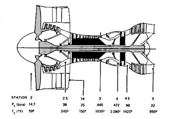
Figure 3.17:
Gas turbine engine
pressures and temperatures
|
|
Figure 3.17 shows pressures
and temperatures through a gas turbine engine (the PW4000, which
powers the 747 and the 767).
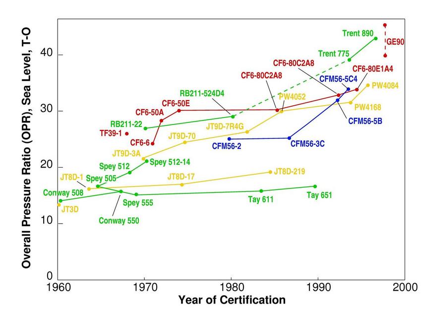
Figure 3.18:
Gas turbine
engine pressure ratio trends (Jane�s Aeroengines, 1998)
|
|
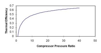
Figure 3.19:
Trend of Brayton cycle thermal efficiency with compressor pressure ratio
|
|
Equation (3.10) says that for a high cycle
efficiency, the pressure ratio of the cycle should be increased.
This trend is plotted in Figure 3.19.
Figure 3.18 shows the history of aircraft
engine pressure ratio versus entry into service, and it can be seen
that there has been a large increase in cycle pressure ratio. The
thermodynamic concepts apply to the behavior of real aerospace
devices!
Muddy Points
When flow is accelerated in a nozzle, doesn't that reduce the
internal energy of the flow and therefore the enthalpy?
(MP 3.11)
Why do we say the combustion in a gas turbine engine is constant
pressure? (MP 3.12)
Why is the Brayton cycle less efficient than the Carnot cycle?
(MP 3.13)
If the gas undergoes constant pressure cooling in the exhaust
outside the engine, is that still within the system boundary?
(MP 3.14)
Does it matter what labels we put on the corners of the cycle or
not? (MP 3.15)
Is the work done in the compressor always equal to the work done in
the turbine plus work out (for a Brayton cyle)?
(MP 3.16)
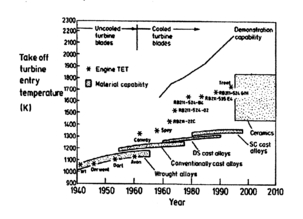
3.7.2 Gas Turbine Technology and Thermodynamics
The turbine entry temperature,  , is fixed by materials
technology and cost. (If the temperature is too high, the blades
fail.) Figures 3.20 and 3.21
show the progression of the turbine entry temperatures in
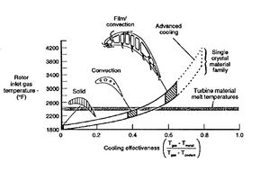
aeroengines. Figure 3.20 is from Rolls Royce and
Figure 3.21 is from Pratt & Whitney. Note the
relation between the gas temperature coming into the turbine blades
and the blade melting temperature.
, is fixed by materials
technology and cost. (If the temperature is too high, the blades
fail.) Figures 3.20 and 3.21
show the progression of the turbine entry temperatures in
aeroengines. Figure 3.20 is from Rolls Royce and
Figure 3.21 is from Pratt & Whitney. Note the
relation between the gas temperature coming into the turbine blades
and the blade melting temperature.
Figure 3.20:
Rolls-Royce high temperature
technology
|
|
Figure 3.21:
Turbine blade cooling
technology [Pratt & Whitney]
|
|
For a given level of turbine technology (in other words given
maximum temperature) a design question is what should the compressor
 be? What criterion should be used to decide this? Maximum
thermal efficiency? Maximum work? We examine this issue below.
be? What criterion should be used to decide this? Maximum
thermal efficiency? Maximum work? We examine this issue below.
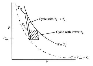
Figure 3.22:
Efficiency and work of two
Brayton cycle engines
|
|
The problem is posed in Figure 3.22, which
shows two Brayton cycles. For maximum efficiency we would like
as high as possible. This means that the compressor exit temperature
approaches the turbine entry temperature. The net work will be less
than the heat received; as
 the heat received
approaches zero and so does the net work.
the heat received
approaches zero and so does the net work.
The net work in the cycle can also be expressed as  ,
evaluated in traversing the cycle. This is the area enclosed by the
curves, which is seen to approach zero as
.
,
evaluated in traversing the cycle. This is the area enclosed by the
curves, which is seen to approach zero as
.
The conclusion from either of these arguments is that a cycle
designed for maximum thermal efficiency is not very useful in that
the work (power) we get out of it is zero.
A more useful criterion is that of maximum work per unit mass
(maximum power per unit mass flow). This leads to compact propulsion
devices. The work per unit mass is given by:
where
is the maximum turbine inlet temperature (a design
constraint) and  is atmospheric temperature. The design
variable is the compressor exit temperature,
is atmospheric temperature. The design
variable is the compressor exit temperature,  , and to find the
maximum as this is varied, we differentiate the expression for work
with respect to
:
, and to find the
maximum as this is varied, we differentiate the expression for work
with respect to
:
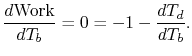
The first and the fourth terms on the right hand side of the above
equation are both zero (the turbine entry temperature is fixed, as
is the atmospheric temperature). The maximum work occurs where the
derivative of work with respect to
is zero:
 |
(3..11) |
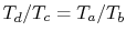
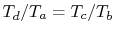
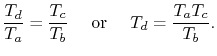
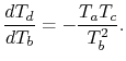
To use Eq. (3.11), we need to relate  and
.
We know that
and
.
We know that
Hence,
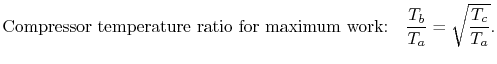
Plugging this expression for the derivative into
Eq. (3.11) gives the compressor exit temperature for
maximum work as
 . In terms of temperature
ratio,
. In terms of temperature
ratio,
The condition for maximum work in a Brayton cycle is different than
that for maximum efficiency. The role of the temperature ratio can
be seen if we examine the work per unit mass which is delivered at
this condition:
Ratioing all temperatures to the engine inlet temperature,
To find the power the engine can produce, we need to multiply the
work per unit mass by the mass flow rate:
![$\displaystyle \textrm{Power} = \dot{m} c_p T_a \left[\frac{T_c}{T_a} -2\sqrt{\frac{T_c}{T_a}}+1\right];\textrm{ Maximum power for an ideal Brayton cycle}.$](img437.png) |
(3..12) |
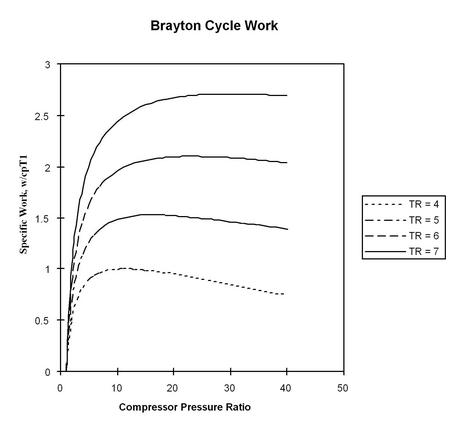
The trend of work output vs. compressor pressure ratio, for
different temperature ratios
 , is shown in
Figure 3.23.
, is shown in
Figure 3.23.
Figure 3.23:
Trend of cycle work with compressor pressure ratio,
for different temperature ratios
|
|
Figure 3.24:
Aeroengine core power [Koff/Meese,
1995]
[Gas turbine engine core]
[Core power vs. turbine entry
temperature]
|
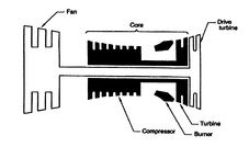
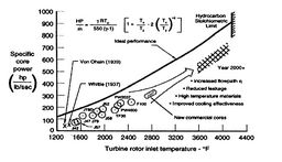
Figure 3.24 shows the expression for power of an ideal
cycle compared with data from actual jet engines.
Figure 3.24(a) shows the gas turbine engine layout including
the core (compressor, burner, and turbine).
Figure 3.24(b) shows the core power for a number of
different engines as a function of the turbine rotor entry
temperature. The equation in the figure for horsepower (HP) is the
same as that which we just derived, except for the conversion
factors. The analysis not only shows the qualitative trend very well
but captures much of the quantitative behavior too.
A final comment (for this section) on Brayton cycles concerns the
value of the thermal efficiency. The Brayton cycle thermal
efficiency contains the ratio of the compressor exit temperature to
atmospheric temperature, so that the ratio is not based on the
highest temperature in the cycle, as the Carnot efficiency is. For a
given maximum cycle temperature, the Brayton cycle is therefore less
efficient than a Carnot cycle.
Muddy Points
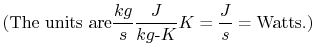
What are the units of  in
in
 ?
(MP 3.17)
?
(MP 3.17)
Question about the assumptions made in the Brayton cycle for maximum
efficiency and maximum work
(MP 3.18)
You said that for a gas turbine engine modeled as a Brayton cycle
the work done is  , where
is the heat added and
is the heat rejected. Does this suggest that the work that you
get out of the engine doesn't depend on how good your compressor and
turbine are?
, where
is the heat added and
is the heat rejected. Does this suggest that the work that you
get out of the engine doesn't depend on how good your compressor and
turbine are? since the compression and expansion were modeled
as adiabatic. (MP 3.19)
since the compression and expansion were modeled
as adiabatic. (MP 3.19)
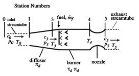
3.7.3 Brayton Cycle for Jet Propulsion: the Ideal Ramjet
A schematic of a ramjet is given in
Figure 3.25.
Figure 3.25:
Ideal ramjet
[J. L. Kerrebrock, Aircraft Engines and Gas Turbines]
|
|
In the ramjet there are ``no moving parts.'' The processes that
occur in this propulsion device are:
-
 : Isentropic diffusion
(slowing down) and compression, with a decrease in Mach number,
: Isentropic diffusion
(slowing down) and compression, with a decrease in Mach number,
 .
.
-
 : Constant pressure combustion.
-
 : Isentropic expansion through the nozzle.
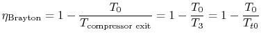
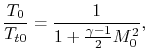
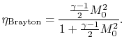
The ramjet thermodynamic cycle efficiency can be written in terms of
flight Mach number,  , as follows:
and
so
See also Section 11.6.3 for other figures of merit.
Muddy Points
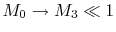
Why don't we like the numbers 1 and 2 for the stations? Why do we go
0-3? (MP 3.20)
For the Brayton cycle efficiency, why does
 ?
(MP 3.21)
?
(MP 3.21)
MIT operates a Brayton cycle power generator on campus. For more
information, see the website at
https://cogen.mit.edu/ctg.cfm
.
UnifiedTP
| 
![$\displaystyle \frac{d\textrm{Work}}{dT_b}= c_p
\left[\frac{dT_c}{dT_b}-1-\frac{dT_d}{dT_b}+\frac{dT_a}{dT_b}
\right].
$](img428.png)
![$\displaystyle \textrm{Work/unit mass }= c_p\left[T_c - \sqrt{T_a T_c}-\frac{T_a
T_c}{\sqrt{T_a T_c}} +T_a\right].
$](img435.png)
![$\displaystyle \textrm{Work/unit mass }= c_p
T_a\left[\frac{T_c}{T_a}-2\sqrt{\frac{T_c}{T_a}}+1\right].
$](img436.png)