Thermodynamics and Propulsion

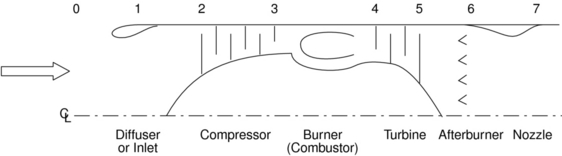
11.6 Performance of Jet Engines

In Chapter 3 we represented a gas turbine engine using a Brayton cycle and derived expressions for efficiency and work as functions of the temperature at various points in the cycle. In this section we will perform further ideal cycle analysis to express the thrust and fuel efficiency of engines in terms of useful design variables, including design limits, flight conditions, and design choices.

The expressions we develop will allow us to define a particular mission and then determine the optimum component characteristics (e.g. compressor, combustor, turbine) for an engine for a given mission. Note that ideal cycle analysis addresses only the thermodynamics of the airflow within the engine. It does not describe the details of the components (the blading, the rotational speed, etc.), but only the results the various components produce (e.g. pressure ratios, temperature ratios). In Chapter 12 we will look in greater detail at how some of the components (the turbine and the compressor) produce these effects.

11.6.1 Notation and station numbering

Notation:

$$T_t = T\left( 1+ \frac{\gamma-1}{2}M^2\right),$$

$$P_t = P\left(1+ \frac{\gamma-1}{2}M^2\right)^\frac{\gamma}{\gamma-1},$$

$$\theta_0 \equiv \frac{T_{t0}}{T_0},$$

$$\theta_T \equiv \frac{T_{t,T}}{T_0},$$

$$\delta_0 \equiv \frac{P_{t0}}{P_0}=\theta_0^\frac{\gamma}{\gamma-1},$$

where the capital subscript $T$ will refer to the turbine. Stagnation properties, $T_t$ and $P_t$ , are more easily measured quantities than static properties ($T$ and $p$ ). Thus, it is standard convention to express the performance of various components in terms of stagnation pressure and temperature ratios:

• $\pi \equiv$ total or stagnation pressure ratio across component ($d$ , $c$ , $b$ , $T$ , $a$ , $n$ )
• $\tau \equiv$ total or stagnation temperature ratio across component ($d$ , $c$ , $b$ , $T$ , $a$ , $n$ ),

where $d = \textrm{diffuser (or inlet)}$ , $c= \textrm{compressor}$ , $b= \textrm{burner (or combustor)}$ , $T= \textrm{turbine}$ , $a= \textrm{afterburner}$ , and $n=\textrm{nozzle}$ . To identify individual stations within the engine we will use the numbers in Figure 11.12.

Figure 11.12: Gas turbine engine station numbering.

11.6.2 Ideal Assumptions

1. Inlet/Diffuser: $\pi_d= 1$ , $\tau_d = 1$ (adiabatic, isentropic)
2. Compressor or fan: $\tau_c = \pi_c^\frac{\gamma-1}{\gamma}$ , $\tau_f = \pi_f^\frac{\gamma-1}{\gamma}$ .
3. Combustor/burner or afterburner: $\pi_b = 1$ , $\pi_a = 1$
4. Turbine: $\tau_T = \pi_T^\frac{\gamma-1}{\gamma}$
5. Nozzle: $\pi_n = 1$ , $\tau_n = 1$ .

11.6.3 Ideal Ramjet

To get started with a simple example (no turbomachinery), we will reexamine the ideal ramjet, picking up where we left off in Section 3.7.3. (Note that we will continue to use station 5 as the exit station, consistent with Figure 3.25.)

11.6.3.1 Thrust

The coordinate system and control volume are chosen to be fixed to the ramjet. The thrust, $F$ , is given by:

$$F = \dot{m}(c_5 - c_0),$$

where $c_5$ and $c_0$ are the exit and inlet flow velocities, respectively. The thrust can be put in terms of nondimensional parameters as follows:

$$\frac{F}{\dot{m}a_0} =\frac{c_5}{a_5}\frac{a_5}{a_0}-\frac{c_0}{a_0},\qquad \textrm{where $a =\sqrt{\gamma RT}$ is the speed of sound,}$$

$$= M_5\frac{a_5}{a_0} -M_0=M_5\sqrt{\frac{T_5}{T_0}}-M_0.$$

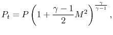
Using $M_3^2$ , $M_4^2 \ll 1$ in the expression for stagnation pressure,

$$\frac{P_t}{P} = \left[1+\frac{\gamma-1}{2}M^2\right]^{\frac{\gamma}{\gamma-1}},$$

$$P_3 \approx P_{t3} = P_{t0};\qquad P_4\approx P_{t4} = P_{t5};\qquad P_4\approx P_3.$$

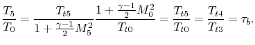
The ratios of stagnation pressure to static pressure at inlet and exit of the ramjet are

$$\underbrace{\frac{P_{t0}}{P_0} = \frac{P_3}{P_0}}_\textrm{determi... ... = \underbrace{\frac{P_4}{P_0} = \frac{P_{te}}{P_e}}_\textrm{determines $M_e$}.$$

The ratios of stagnation to static pressure at exit and at inlet are the same, with the consequence that the inlet and exit Mach numbers are also the same.

$$M_5 = M_0.$$

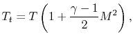
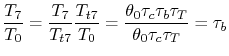
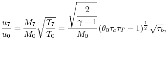
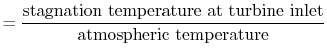
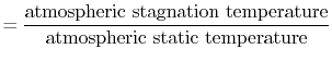
To find the thrust we need to find the ratio of the temperature at exit and the temperature at inlet. This is given by

$$\frac{T_5}{T_0} = \frac{T_{t5}}{1+\frac{\gamma-1}{2}M_5^2} \frac{... ...{\gamma-1}{2}M_0^2}{T_{t0}}=\frac{T_{t5}}{T_{t0}}=\frac{T_{t4}}{T_{t3}}=\tau_b.$$

where $\tau_b$ is the stagnation temperature ratio across the combustor (burner). The thrust is thus

$$\frac{F}{\dot{m}a_0} =M_0(\sqrt{\tau_b} -1).$$

11.6.3.2 Fuel Air Ratio

To find the Isp will will need to find the ramjet fuel-air ratio, $f$ . Using a control volume around the burner, as shown in Figure 11.13, we get:

$$\textrm{Heat given to the fluid: }\quad \dot{Q} = \dot{m}_f \Delta h_\textrm{fuel} = \dot{m} f \Delta h_\textrm{fuel}.$$

From the steady flow energy equation:

$$\dot{m}_4h_{t4} - \dot{m}_3h_{t3}=\dot{m}_3f\Delta h_\textrm{fuel}.$$

The exit mass flow is not greatly different from the inlet mass flow, $\dot{m}_4 = \dot{m}_3(1+f) \approx \dot{m}_3$ , because the fuel-air ratio is much less than unity (generally several percent). We thus neglect the difference between the mass flows and obtain

$$h_{t4} - h_{t3} = c_p (T_{t4} - T_{t3})= f \Delta h_\textrm{fuel},$$

$$T_{t3} c_p(\tau_b-1) = f \Delta h_\textrm{fuel},$$

with

$$T_{t3} = T_{t0} = T_0 \underbrace{\left(1+\frac{\gamma-1}{2}M_0^2\right)}_{\Theta_0}.$$

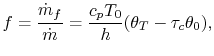
Thus, the fuel-air ratio is

$$f = \frac{\tau_b-1}{\Delta h_\textrm{fuel}/c_p T_0 \Theta_0}.$$

The fuel-air ratio, $f$ , depends on the fuel properties ( $\Delta h_\textrm{fuel}$ ), the desired flight parameters ($\Theta_0$ ), the ramjet performance ($\tau_b$ ), and the temperature of the atmosphere ($T_0$ ).

Figure 11.13: Control volume over the burner

11.6.3.3 Specific impulse, $I_{sp}$

The specific impulse for the ramjet is given by

$$I_{sp} = \frac{F}{f \dot{m} g} = \frac{1}{g} \frac{(\sqrt{\tau_b}-1)\left(c_0 \Delta h_\textrm{fuel}/c_pT_0\right)} {\Theta_0(\tau_b-1)}.$$

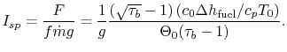
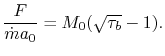
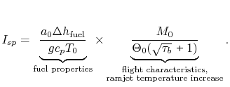
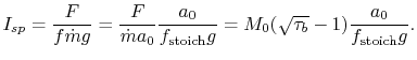
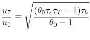
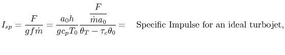
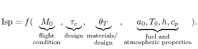
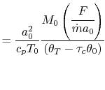
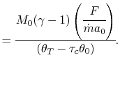
The specific impulse can be written in terms of fuel properties and flight and vehicle characteristics as

$$I_{sp} = \underbrace{\frac{a_0\Delta h_\textrm{fuel}}{g c_p T_0}}... ...ack{\textrm{flight characteristics,}\\ \textrm{ramjet temperature increase}}}.$$

We wish to explore the parameter dependency of the above expression, which is a complicated formula. How can we do this? What are the important effects of the different parameters? How do we best capture the ramjet performance behavior?

To make effective comparisons, we need to add some additional information concerning the operational behavior. An important case to examine is when we have stoichiometric conditions and all the fuel burns (denoted by $f_\textrm{stoich}$ ). What happens in this situation as the flight Mach number, $M_0$ , increases? $T_0$ is fixed so $T_{t3}$ increases, but the maximum temperature does not increase much because of dissociation: the reaction does not go to completion at high temperature. A useful approximation is therefore to take $T_{t4}$ constant for stoichiometric operation. In the stratosphere, from 10 to 30 km, $T_0 \approx \textrm{constant} \approx 212\textrm{ K}$ . 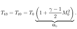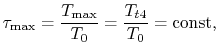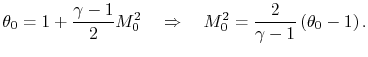The maximum temperature ratio is

$$\tau_\textrm{max}= \frac{T_\textrm{max}}{T_0}= \frac{T_{t4}}{T_0} = \textrm{const},$$

$$\tau_b = \frac{T_{t4}}{T_{t3}}=\frac{T_{t4}/T_0}{T_{t3}/T_0}=\frac{\tau_\textrm{max}}{\Theta_0}.$$

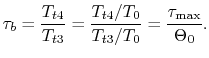
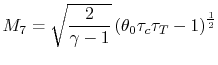
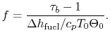
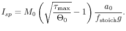
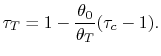
For the stoichiometric ramjet,

$$I_{sp} =\frac{F}{f \dot{m}g}=\frac{F}{\dot{m}a_0}\frac{a_0}{f_\textrm{stoich}g}=M_0(\sqrt{\tau_b} - 1)\frac{a_0}{f_\textrm{stoich}g}.$$

Using the expression for $\tau_b$ , the specific impulse is

$$I_{sp} = M_0\left(\sqrt{\frac{\tau_\textrm{max}}{\Theta_0}}-1\right)\frac{a_0}{f_\textrm{stoich}g}.$$

11.6.3.4 Representative performance values

Figure 11.14: Thrust per unit mass flow and specific impulse for ideal ramjet with stoichiometric combustion [Kerrebrock]

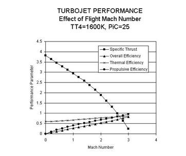
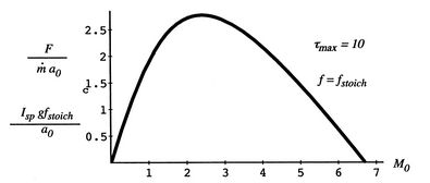
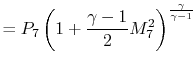
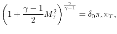
A plot of the performance of the stoichiometric ramjet is shown in Figure 11.14. The figure shows that for the parameters used, the best operating range of a hydrocarbon-fueled ramjet is $2 \leq M_0 \leq 4$ . The parameters used are $\tau_\textrm{max} = 10$ , $a_0 \approx 300\textrm{ m/s}$ in the stratosphere, $f_\textrm{stoich} = 0.067$ for hydrocarbons, such that $a_0/g f_\textrm{stoich} \approx 450\textrm{ s}$ .

11.6.3.5 Recapitulation

Between Section 3.7.3 and this section we have:

• Examined the Brayton Cycle for ramjet propulsion,
• Found $\eta_\textrm{Brayton}$ as a function of $M_0$ ,
• Found $\eta_\textrm{overall}$ and the relation between $\eta_{overall}$ and $\eta_\textrm{Brayton}$ , and
• Examined $F/\dot{m}a_0$ and $I_{sp}$ as a function of $M_0$ .

Muddy Points What exactly is the specific impulse, $I_{sp}$ , a measure of? (MP 11.1)

How is $I_{sp}$ found for rockets in space where $g \approx 0$ ? (MP 11.2)

Why does industry use $TSFC$ rather than $I_{sp}$ ? Is there an advantage to this? (MP 11.3)

Why isn't mechanical efficiency an issue with ramjets? (MP 11.4)

How is thrust created in a ramjet? (MP 11.5)

What is the relation between $h_{t4} - h_{t3} = f\Delta h_f$ and the existence of the maximum value of $T_{t4}$ ? (MP 11.6)

Why didn't we have a 2s point for the Brayton cycle with non-ideal components? (MP 11.7)

What is the variable $f_\textrm{stoich}$ ? (MP 11.8)

11.6.4 Turbojet Engine

Figure 11.15: Schematic with appropriate component notations added.

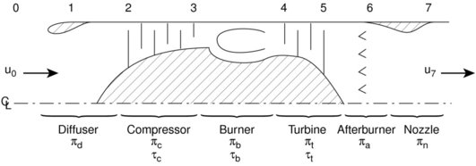
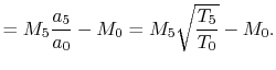
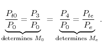
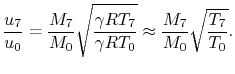
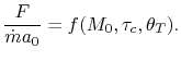
We now examine an engine with turbomachinery, as shown in Figure 11.15. Methodology:

1. Find thrust by finding $u_{\textrm{exit}/}u_0$ in terms of $\theta_0$ , temperature ratios, etc.
2. Use a power balance to relate turbine parameters to compressor parameters
3. Use an energy balance across the combustor to relate the combustor temperature rise to the fuel flow rate and fuel energy content.

First write-out the expressions for thrust and Isp:

$$F = \dot{m} [(1+ f)u_7 - u_0]+(p_7-p_0)A_7,$$

where $f$ is the fuel/air mass flow ratio,

$$F = \dot{m}(u_7-u_0) \quad \Rightarrow \quad \frac{F}{\dot{m}a_0} = M_0\left[\frac{u_7}{u_0}-1\right] \quad \textrm{(can neglect fuel)},$$

and

$$\textrm{Isp} = \frac{F}{\dot{m}_f g} = \frac{F}{g f \dot{m}}.$$

Now we have to do a little algebra to manipulate these expressions into more useful forms. First we write an expression for the exit velocity:

$$\frac{u_7}{u_0} = \frac{M_7}{M_0}\sqrt{\frac{\gamma R T_7}{\gamma R T_0}}\approx \frac{M_7}{M_0}\sqrt{\frac{T_7}{T_0}}.$$

Noting that

$$\frac{T_{t7}}{T_7} =T\left(1+ \frac{\gamma-1}{2}M_7^2\right),$$

we can write

$$T_{t7} = T_{t0}\left(\frac{T_{t2}}{T_{t0}}\right) \left(\frac{T_{t3}}{T_... ...3}}\right) \left(\frac{T_{t5}}{T_{t4}}\right)\left(\frac{T_{t7}}{T_{t5}}\right)$$

$$=T_{t0}(\tau_d \tau_c \tau_b \tau_T \tau_n)$$

$$= T_0\left(1+\frac{\gamma-1}{2}M_0^2\right)\tau_c\tau_b\tau_T.$$

Thus

$$T_{t7} = T_0 \theta_0 \tau_c \tau_b \tau_T,$$ (11..1)

which expresses the exit temperature as a function of the inlet temperature, the Mach number, and the temperature changes across each component. We now write the pressure at the exit in a similar manner:

$$P_{t7} = P_0\left(1 +\frac{\gamma-1}{2}M_0^2\right)^\frac{\gamma}{\gamma-1} \pi_d\pi_c\pi_b\pi_T\pi_n$$

$$= p_0 \delta_0 \pi_c \pi_T.$$

Since

$$P_{t7} = P_7 \left(1+\frac{\gamma-1}{2}M_7^2\right)^\frac{\gamma}{\gamma-1}$$
and

$$p_7 = p_0$$

we write

$$\left(1+\frac{\gamma-1}{2}M_7^2\right)^\frac{\gamma}{\gamma-1} = \delta_0 \pi_c \pi_T,$$

and then equate this to our expression for the temperature in (11.1):

$$1+\frac{\gamma-1}{2}M_7^2 = \delta_0^\frac{\gamma-1}{2}\pi_c^\fra... ...T^\frac{\gamma-1}{2} = \theta_0 \tau_c \tau_T \left(=\frac{T_{t7}}{T_7}\right),$$

and

$$M_7 = \sqrt{\frac{2}{\gamma-1}}\left(\theta_0 \tau_c \tau_T -1\right)^\frac{1}{2}$$

We now continue on the path to our expression for $u_7/u_0$ .

$$\frac{T_7}{T_0} = \frac{T_7}{T_{t7}}\frac{T_{t7}}{T_0} = \frac{\theta_0 \tau_c \tau_b \tau_T}{\theta_0 \tau_c \tau_T} = \tau_b$$

$$\frac{u_7}{u_0} = \frac{M_7}{M_0}\sqrt{\frac{T_7}{T_0}} = \cfrac{... ...amma-1}}}{M_0} \left(\theta_0 \tau_c \tau_T -1\right)^\frac{1}{2}\sqrt{\tau_b},$$

$$\theta_0 = 1 +\frac{\gamma-1}{2}M_0^2 \quad \Rightarrow \quad M_0^2 = \frac{2}{\gamma-1}\left(\theta_0 - 1\right).$$

Therefore

$$\frac{u_7}{u_0} = \sqrt{\frac{(\theta_0 \tau_c \tau_T -1)\tau_b}{\theta_0-1}}$$

Now we have two steps left. First we write $\tau_c$ in terms of $\tau_T$ , by noting that they are related by the condition that the power used by the compressor is equal to the power extracted by the turbine. Second, we put the burner temperature ratio in terms of the exit temperature of the burner, ($T_{t4}$ or more specifically $\theta_T = T_{t4}/T_0$ ) since this is the hottest point in the engine and is a frequent benchmark used for judging various designs.

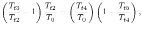
The steady flow energy equation states

$$\dot{m} \Delta h_t = \dot{q} - \dot{w}_s.$$

Assuming that the compressor and turbine are adiabatic, then

$$\dot{m}\Delta h_t = -\textrm{rate of shaft work done by the system}=\textrm{rate of shaft work done on the system}.$$

Since the turbine shaft is connected to the compressor shaft

$$\dot{m}_c c_{p,c} (T_{t3} - T_{t2}) = \dot{m}_T c_{p,T}(T_{t4} - T_{t5})$$

Assuming the mass flow and specific heats are the same between compressor and turbine, this can be rewritten as

$$\left(\frac{T_{t3}}{T_{t2}}-1\right)\frac{T_{t2}}{T_0} = \left(\frac{T_{t4}}{T_0}\right)\left(1-\frac{T_{t5}}{T_{t4}}\right),$$

where

$$\frac{T_{t2}}{T_0} = \tau_d \theta_0 = \theta_0,$$

so

$$(\tau_c-1)\theta_0 = \theta_T(1-\tau_T)$$

or

$$\tau_T = 1 - \frac{\theta_0}{\theta_T}(\tau_c-1).$$

That was the first step relating the temperature rise across the turbine to that across the compressor. The remaining step is to write the temperature rise across the combustor in terms of $\theta_t =T_{t4}/T_0$ .

$$\tau_b = \frac{\theta_T}{\theta_0 \tau_c}$$

and for an engine with an afterburner

$$\tau_b = \frac{\theta_a}{\theta_T \tau_T}.$$

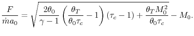
Now substituting our expressions for $\tau_b$ , and $\tau_T$ into our expression for $u_7/u_0$ , and finally into the first expression we wrote for thrust, we get:

$$\frac{F}{\dot{m}a_0} = M_0\left[\left\{\left(\frac{\theta_0}{\the... ..._c} \right\}^\frac{1}{2}-1\right] \quad \textrm{Specific thrust for a turbojet}$$

This is what we were seeking, an expression for thrust in terms of important design parameters and flight parameters:

$$\frac{F}{\dot{m}a_0} = f(M_0,\tau_c,\theta_T).$$

By adding and substracting the quantity

$$\frac{2\theta}{\gamma-1}\left(\frac{\theta_T}{\theta_0 \tau_c}\right),$$

we may write this write in another form which is often used,

$$\frac{F}{\dot{m}a_0} = \sqrt{\frac{2\theta_0}{\gamma-1}\left(\fra... ...{\theta_0\tau_c}-1\right)(\tau_c-1)+\frac{\theta_T M_0^2}{\theta_0\tau_c}}-M_0.$$

A recap of the important variables:

$$\tau_c = \textrm{temperature ratio across compressor}$$

$$\theta_T = \frac{\textrm{stagnation temperature at turbine inlet}}{\textrm{atmospheric temperature}}$$

$$\theta_0 = \frac{\textrm{atmospheric stagnation temperature}}{\textrm{atmospheric static temperature}}$$

$$a_0 = \textrm{speed of sound}$$

$$F = \textrm{thrust}.$$

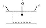
Our final step involves writing the specific impulse and other measures of efficiency in terms of these same parameters. We begin by writing the First Law across the combustor to relate the fuel flow rate and heating value of the fuel to the total enthalpy rise.

$$\dot{m}_f h = \dot{m}c_p(T_{t4}-T_{t3})$$

and

$$f=\frac{\dot{m}_f}{\dot{m}}=\frac{c_p T_0}{h}(\theta_T - \tau_c\theta_0),$$

where again, $f$ is the fuel/air mass flow ratio. The specific impulse becomes

$$I_{sp} = \frac{F}{g f\dot{m}} = \frac{a_0 h}{g c_p T_0}\cfrac{\cf... ...\theta_T-\tau_c\theta_0}=\quad \textrm{Specific Impulse for an ideal turbojet},$$

where $I_{sp}$ is expressed in terms of typical design parameters, flight conditions, and physical constants

$$\textrm{Isp} = f(\underbrace{M_0}_{\substack{\textrm{flight} \t... ...0,T_0,h,c_p}_{\substack{\textrm{fuel and} \textrm{atmospheric properties}}}).$$

Similarly, we can write our overall efficiency as

$$\eta_{\textrm{overall}} = \frac{F u_0}{\dot{m}_f h}$$

$$= \frac{a_0^2}{c_p T_0}\cfrac{M_0\left(\cfrac{F}{\dot{m}a_0}\right)}{(\theta_T-\tau_c\theta_0)}$$
or

$$\eta_{\textrm{overall}} = \cfrac{M_0(\gamma-1)\left(\cfrac{F}{\dot{m}a_0}\right)}{(\theta_T-\tau_c\theta_0)}.$$

Using the definition from before, the ideal thermal efficiency is

$$\eta_{\textrm{thermal}} = 1 - \frac{1}{\theta_0 \tau_c},$$

and the propulsive efficiency can be found as

$$\eta_{\textrm{propulsive}} =\frac{\eta_{\textrm{overall}}}{\eta_{\textrm{thermal}}}.$$

We can now use these equations to better understand the performance of a simple turbojet engine. We will use the following parameters (with $\gamma= 1.4$ ):

Table 11.1: Turbojet Mission Parameters

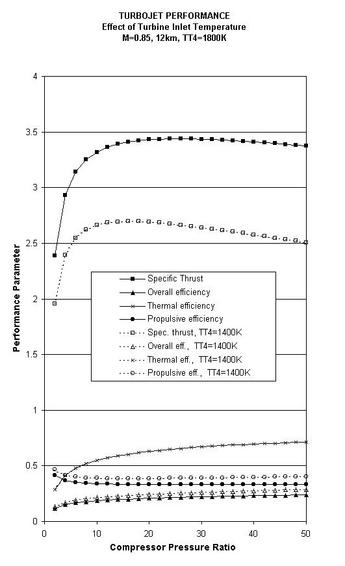
Mach number	Altitude	Ambient Temp.	Speed of sound
0	Sea level	288 K	340 m/s
0.85	12 km	217 K	295 m/s
2.0	18 km	217 K	295 m/s

Note it is more typical to work with the compressor pressure ratio ($\pi_c$ ) rather than the temperature ratio ($\tau_c$ ) so we will substitute the isentropic relationship:

$$\tau_c = \pi_c ^\frac{\gamma-1}{\gamma}$$

into the equations before plotting the results in Figures 11.16, 11.17, and 11.18.

Figure 11.16: Performance of an ideal turbojet engine as a function of flight Mach number.

Figure 11.17: Performance of an ideal turbojet engine as a function of compressor pressure ratio and flight Mach number.

Figure 11.18: Performance of an ideal turbojet engine as a function of compressor pressure ratio and turbine inlet temperature.

11.6.5 Effect of Departures from Ideal Behavior -- Real Cycle behavior

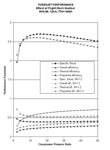
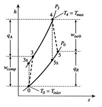
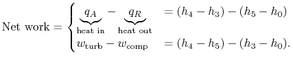
To conclude this chapter, we will now improve our estimates of cycle performance by including the effects of irreversibility. We will use the Brayton cycle as an example. What are the sources of non-ideal performance and departures from reversibility?

• Losses (entropy production) in the compressor and the turbine.
• Stagnation pressure decrease in the combustor.
• Heat transfer.

We take into account here only irreversibility in the compressor and in the turbine. Because of these irreversibilities, we need more work, $\Delta h_\textrm{comp}$ (the changes in kinetic energy from inlet to exit of the compressor are neglected), to drive the compressor than in the ideal situation. We also get less work, $\Delta h_\textrm{turb}$ , back from the turbine. The consequence, as can be inferred from Figure 11.19, is that the net work from the engine is less than in the cycle with ideal components.

Figure 11.19: Gas turbine engine (Brayton) cycle showing effect of departure from ideal behavior in compressor and turbine

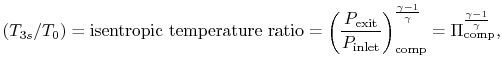
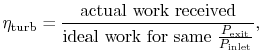
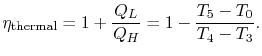
To develop a quantitative description of the effect of these departures from reversible behavior, consider a perfect gas with constant specific heats and neglect kinetic energy at the inlet and exit of the turbine and compressor. We define the turbine adiabatic efficiency as

$$\eta_\textrm{turb} = \frac{w_\textrm{turb}^\textrm{actual}}{w_\textrm{turb}^\textrm{ideal}} = \frac{h_4-h_5}{h_4-h_{5s}},$$

where $w_\textrm{turb}^\textrm{actual}$ is specified to be at the same pressure ratio as $w_\textrm{turb}^\textrm{ideal}$ . There is a similar metric for the compressor, the compressor adiabatic efficiency:

$$\eta_\textrm{comp} = \frac{w_\textrm{comp}^\textrm{ideal}}{w_\textrm{comp}^\textrm{actual}} = \frac{h_{3s}-h_0}{h_3-h_0},$$

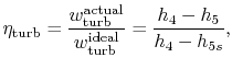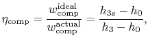
again for the same pressure ratio. Note that for the turbine the ratio is the actual work delivered divided by the ideal work, whereas for the compressor the ratio is the ideal work needed divided by the actual work required. These are not thermal efficiencies, but rather measures of the degree to which the compression and expansion approach the ideal processes.

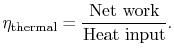
We now wish to find the net work done in the cycle and the efficiency. The net work is given either by the difference between the heat received and rejected or the work of the compressor and turbine, where the convention is that heat received is positive and heat rejected is negative and work done is positive and work absorbed is negative.

$$\textrm{Net work}=\begin{cases}\underbrace{q_A}_\textrm{heat in} ... ...0) w_\textrm{turb} - w_\textrm{comp} &= (h_4 - h_5) - (h_3 -h_0). \end{cases}$$

The thermal efficiency is

$$\eta_\textrm{thermal} = \frac{\textrm{Net work}}{\textrm{Heat input}}.$$

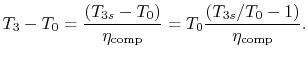
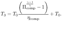
We need to calculate $T_3$ , $T_5$ .

From the definition of $\eta_\textrm{comp}$ ,

$$T_3 - T_0 =\frac{(T_{3s} - T_0)}{\eta_\textrm{comp}}= T_0\frac{( T_{3s}/T_0 - 1)}{\eta_\textrm{comp}}.$$

With

$$(T_{3s}/T_0)= \textrm{isentropic temperature ratio} = \left(\frac... ...{comp}^{\frac{\gamma-1}{\gamma}} = \Pi_\textrm{comp}^{\frac{\gamma-1}{\gamma}},$$

$$T_3=T_0\frac{\left(\Pi_\textrm{comp}^{\frac{\gamma-1}{\gamma}}-1\right)}{\eta_\textrm{comp}}+T_0.$$

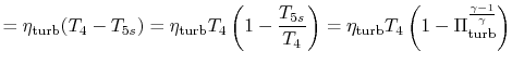
Similarly, by the definition

$$\eta_\textrm{turb} = \frac{\textrm{actual work received}} {\textrm{ideal work for same $\frac{P_\textrm{exit}}{P_\textrm{inlet}}$}},$$

we can find $T_5$ :

$$T_4-T_5 = \eta_\textrm{turb}(T_4-T_{5s}) = \eta_\textrm{turb}T_4\left(1-\... ... =\eta_\textrm{turb}T_4\left(1-\Pi_\textrm{turb}^\frac{\gamma-1}{\gamma}\right)$$

$$T_5 =T_4-\eta_\textrm{turb}T_4\left(1-\Pi_\textrm{turb}^\frac{\gamma-1}{\gamma}\right).$$

The thermal efficiency can now be found:

$$\eta_\textrm{thermal} = 1 + \frac{Q_L}{Q_H} = 1 - \frac{T_5-T_0}{T_4-T_3}.$$

With

$$\Pi_\textrm{comp} = \frac{1}{\Pi_\textrm{turb}} = \Pi$$
and

$$\tau_s = \Pi^{\frac{\gamma-1}{\gamma}} = \textrm{the isentropic cycle temperature ratio},$$

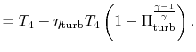
$$\eta_\textrm{thermal} = 1-\cfrac{T_4\left[1-\eta_\textrm{turb}\left(1-\cfrac{1}{\tau_s}... ...ht)\right]-T_0} {T_4-T_0\left[\cfrac{1}{\eta_\textrm{comp}}(\tau_s-1)+1\right]}$$
or

$$\eta_\textrm{thermal} = \frac{\left[1-\cfrac{1}{\tau_s}\right]\left[\eta_\textrm{comp}\... ...0}-\tau_s\right]} {1+\eta_\textrm{comp}\left[\cfrac{T_4}{T_0}-1\right]-\tau_s}.$$

There are several non-dimensional parameters that appear in this expression for thermal efficiency. We list these in the two sections below and show their effects in accompanying figures.

11.6.5.1 Parameters reflecting design choices

$$\Pi : \textrm{cycle pressure ratio}$$

$$\frac{T_4}{T_0} : \textrm{maximum turbine inlet temperature}$$

11.6.5.2 Parameters reflecting the ability to design and execute efficient components

$$\eta_\textrm{comp} :\textrm{compressor adiabatic efficiency}$$

$$\eta_\textrm{turb} :\textrm{turbine adiabatic efficiency}$$

In addition to efficiency, net rate of work is a quantity we need to examine,

$$\dot{W}_\textrm{net} =\dot{W}_\textrm{turbine} -\dot{W}_\textrm{compressor}.$$

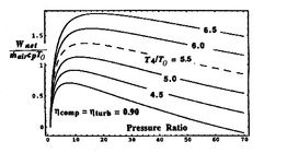
Putting this in a non-dimensional form,

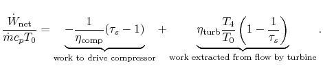
$$\frac{\dot{W}_\textrm{net}}{\dot{m} c_p T_0} = \underbrace{-\frac... ...\left(1-\frac{1}{\tau_s}\right)} _\textrm{work extracted from flow by turbine}.$$

$$\frac{\dot{W}_\textrm{net}}{\dot{m}c_pT_0} = (\tau_s-1)\left[\cfrac{\eta_\textrm{turb}\cfrac{T_4}{T_0}}{\tau_s}-\frac{1}{\eta_\textrm{comp}}\right]$$

Figure 11.20: Non-dimensional power and efficiency for a non-ideal gas turbine engine [from Cumpsty, Jet Propulsion]

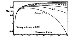
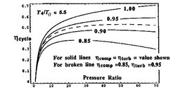
[Non-dimensional work as a function of cycle pressure ratio for different values of turbine entry temperature divided by compressor entry temperature] [Overall cycle efficiency as a function of pressure ratio for different values of turbine entry temperature divided by compressor entry temperature] [Overall cycle efficiency as a function of cycle pressure ratio for different component efficiencies]

Trends in net power and efficiency are shown in Figure 11.20 for parameters typical of advanced civil engines. Some points to note in the figure:

• For any $\eta_\textrm{comp}$ , $\eta_\textrm{turb} \neq 1$ the optimum pressure ratio $(\Pi)$ for maximum $\eta_\textrm{th}$ is not the highest that can be achieved, as it is for the ideal Brayton cycle. The ideal analysis is too idealized in this regard. The highest efficiency also occurs closer to the pressure ratio for maximum power than in the case of an ideal cycle. Choosing this as a design criterion will therefore not lead to the efficiency penalty inferred from ideal cycle analysis.
• There is a strong sensitivity to the component efficiencies. For example, for $\eta_\textrm{turb}=\eta_\textrm{comp}= 0.85$ , the cycle efficiency is roughly two-thirds of the ideal value.
• The maximum power occurs at a value of $\tau_s$ or pressure ratio $(\Pi)$ less than that for max $\eta$ (this trend is captured by ideal analysis).
• The maximum power and maximum $\eta_\textrm{thermal}$ are strongly dependent on the maximum temperature, $T_4/T_0$ .

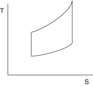
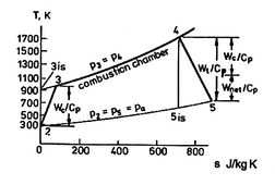
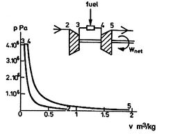
A scale diagram of a Brayton cycle with non-ideal compressor and turbine behaviors, in terms of temperature-entropy ($h$ -$s$ ) and pressure-volume ($P$ -$v$ ) coordinates is given below as Figure 11.21.

Figure 11.21: Scale diagram of non-ideal gas turbine cycle. Nomenclature is shown in the figure. Pressure ratio $40$ , $T_0 = 288\textrm{ K}$ , $T_4 =1700\textrm{ K}$ , compressor and turbine efficiencies $= 0.9$ [from Cumpsty, Jet Propulsion]

[] []

Muddy Points

Isn't it possible for the mixing of two gases to go from the final state to the initial state? If you have two gases in a box, they should eventually separate by density, right? (MP 11.9)

How can $T_4/T_0$ be the maximum turbine inlet temperature? (MP 11.10)

When there are losses in the turbine that shift the expansion in $T$ -$s$ diagram to the right, does this mean there is more work than ideal since the area is greater? (MP 11.11)

For an afterburning engine, why must the nozzle throat area increase if the temperature of the fluid is increased? (MP 11.12)

Why doesn't the pressure in the afterburner go up if heat is added? (MP 11.13)

Why is the flow in the nozzle choked? (MP 11.14)

What's the point of having a throat if it creates a retarding force? (MP 11.15)

Why isn't the stagnation temperature conserved in this steady flow? (MP 11.16)