18.3 Transient Heat Transfer (Convective Cooling or Heating)
All the heat transfer problems we have examined have been steady
state, but there are often circumstances in which the
transient response to heat transfer is critical. An example
is the heating up of gas turbine compressors as they are brought up
to speed during take-off. The disks that hold the blades are large
and take a long time to come to temperature, while the casing is
thin and in the path of high velocity compressor flow and thus comes
to temperature rapidly. The result is that the case expands away
from the blade tips, sometimes enough to cause serious difficulties
with aerodynamic performance.
To introduce the topic as well as to increase familiarity with
modeling of heat transfer problems, we examine a lumped
parameter analysis of an object cooled by a stream. This will allow
us to see what the relevant non-dimensional parameters are and, at
least in a qualitative fashion, how more complex heat transfer
objects will behave. We want to view the object as a ``lump''
described by a single parameter. We need to determine when this type
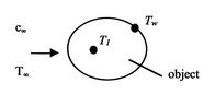
of analysis would be appropriate. To address this, consider the
temperature difference  between two locations in the
object, as shown in Figure 18.6.
between two locations in the
object, as shown in Figure 18.6.
Figure 18.6:
Temperature variation in
an object cooled by a flowing fluid
|
|
If the heat transfer within the body and from the body to the fluid
are of the same magnitude,
where  is a relevant length scale, say half the thickness of the
object. The ratio of the temperature difference is
is a relevant length scale, say half the thickness of the
object. The ratio of the temperature difference is
 |
(18..14) |
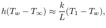
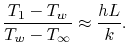
If the Biot number is small the ratio of temperature differences
described in Equation (18.14) is also
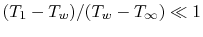 . We can thus say
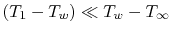 and neglect the temperature non-uniformity within
the object.
and neglect the temperature non-uniformity within
the object.
The approximation made is to view the object as having a spatially
uniform temperature that is a function of time only. Explicitly,  . The first law applied to the object is (using the fact that
for solids
. The first law applied to the object is (using the fact that
for solids
 ),
),
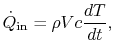 |
(18..15) |
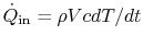
where  is the density of the object and
  is its volume. In
terms of heat transferred to the fluid,
is its volume. In
terms of heat transferred to the fluid,
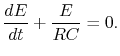
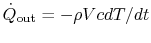 . The rate of heat transfer to the fluid is
 , so the expression for the time evolution of the
temperature is
, so the expression for the time evolution of the
temperature is
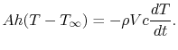 |
(18..16) |
The initial temperature,  , is equal to some known value, which
we can call
, is equal to some known value, which
we can call  . Using this, Equation (18.16)
can be written in terms of a non-dimensional temperature difference
. Using this, Equation (18.16)
can be written in terms of a non-dimensional temperature difference
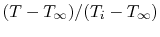 ,
,
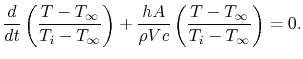 |
(18..17) |
At time  , this non-dimensional quantity is equal to one.
Equation (18.17) is an equation you have
seen before,
, this non-dimensional quantity is equal to one.
Equation (18.17) is an equation you have
seen before,
 which has
the solution
which has
the solution
 . For the present problem the form
is
. For the present problem the form
is
 |
(18..18) |
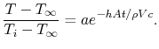
The constant  can be seen to be equal to unity to satisfy the
initial condition. This form of equation implies that the solution
has a heat transfer ``time constant'' given by
can be seen to be equal to unity to satisfy the
initial condition. This form of equation implies that the solution
has a heat transfer ``time constant'' given by
 .
.
The time constant,  , is in accord with our intuition, or
experience; high density, large volume, or high specific heat all
tend to increase the time constant, while high heat transfer
coefficient and large area will tend to decrease the time constant.
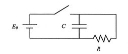
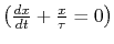
This is the same form of equation and the same behavior you have
seen for the R-C circuit, as shown schematically in
Figure 18.7. The time
dependence of the voltage in the R-C circuit when the switch is
opened suddenly is given by the equation
, is in accord with our intuition, or
experience; high density, large volume, or high specific heat all
tend to increase the time constant, while high heat transfer
coefficient and large area will tend to decrease the time constant.
This is the same form of equation and the same behavior you have
seen for the R-C circuit, as shown schematically in
Figure 18.7. The time
dependence of the voltage in the R-C circuit when the switch is
opened suddenly is given by the equation
There are, in fact, a number of physical processes which have (or
can be modeled as having) this type of exponentially decaying
behavior.
Figure 18.7:
Voltage change
in an R-C circuit
|
|
Muddy Points
In equation
 (18.15), what is
  ?
(MP 18.5)
?
(MP 18.5)
In the lumped parameter transient heat transfer problem, does a high
density ``slow down'' heat transfer?
(MP 18.6)
UnifiedTP
|