
|
|
|
| Thermodynamics and Propulsion | |
|
Next: 8.4 The Clausius-Clapeyron Equation Up: 8. Power Cycles with Previous: 8.2 Work and Heat Contents Index
|
|
[cycle in 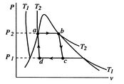 [cycle in
 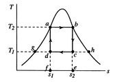 [cycle in
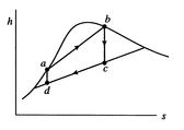
|
A Carnot cycle that uses a two-phase fluid as the working medium is
shown below in Figure 8.7.
Figure 8.7(a) gives the cycle in ![]() -
-![]() coordinates, Figure 8.7(b) in
coordinates, Figure 8.7(b) in ![]() -
-![]() coordinates, and Figure 8.7(c) in
coordinates, and Figure 8.7(c) in ![]() -
-![]() coordinates. The boundary of the region in which there is liquid and
vapor both present (the vapor dome) is also indicated. Note that the
form of the cycle is different in the
coordinates. The boundary of the region in which there is liquid and
vapor both present (the vapor dome) is also indicated. Note that the
form of the cycle is different in the ![]() -
-![]() and
and ![]() -
-![]() representation; it is only for a perfect gas with constant specific
heats that cycles in the two coordinate representations have the
same shapes.
representation; it is only for a perfect gas with constant specific
heats that cycles in the two coordinate representations have the
same shapes.
The processes in the cycle are as follows:
In the ![]() -
-![]() diagram the heat received,
diagram the heat received, ![]() , is
, is ![]() and the
heat rejected,
and the
heat rejected, ![]() , is
, is ![]() . The net work is represented by
. The net work is represented by
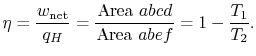
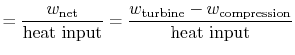
![]() . The thermal efficiency is given by
. The thermal efficiency is given by
In the
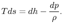
For a constant pressure reversible process,

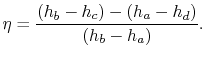
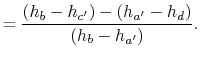
The heat received and rejected per unit mass is given in terms of the enthalpy at the different states as
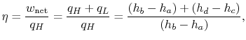
or, in terms of the work done during the isentropic compression and expansion processes, which correspond to the shaft work done on the fluid and received by the fluid,
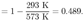
What is the (i) thermal efficiency and (ii) ratio of turbine work to compression (pump) work if
 |
||
 |
To find the work in the pump (compression process) or in the
turbine, we need to find the enthalpy changes between states ![]() and
and
![]() ,
,
![]() , and the change between
, and the change between ![]() and
and ![]() ,
,
![]() . To obtain these the approach is to use the fact that
. To obtain these the approach is to use the fact that
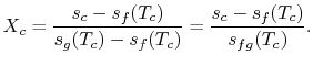
![]() during the expansion to find the quality at
state
during the expansion to find the quality at
state ![]() and then, knowing the quality, calculate the enthalpy as
and then, knowing the quality, calculate the enthalpy as
![]() . We know the conditions at state
. We know the conditions at state ![]() , where
the fluid is all vapor, i.e., we know
, where
the fluid is all vapor, i.e., we know ![]() ,
, ![]() ,
, ![]() :
:
We know:
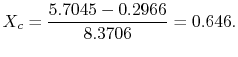
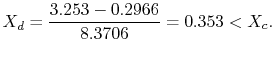
The quality at state ![]() is thus,
is thus,
The enthalpy at state
Substituting the values,
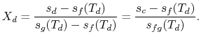
We can apply a similar process to find the conditions at state
We have given that
The enthalpy at state
The ratio of turbine work to compression work (pump work) is
We can check the efficiency by computing the ratio of net work
We can find the turbine work using the definition of turbine and compressor adiabatic efficiencies. The relation between the enthalpy changes is
Substituting the numerical values, the turbine work per unit mass is
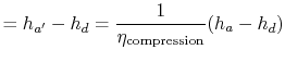
For the compression process, we use the definition of compressor (or pump) adiabatic efficiency:
 |
||
 |
||
 |
A question arises as to whether the Carnot cycle can be practically applied for power generation. The heat absorbed and the heat rejected both take place at constant temperature and pressure within the two-phase region. These can be closely approximated by a boiler for the heat addition process and a condenser for the heat rejection. Further, an efficient turbine can produce a reasonable approach to reversible adiabatic expansion, because the steam is expanded with only small losses. The difficulty occurs in the compression part of the cycle. If compression is carried out slowly, there is equilibrium between the liquid and the vapor, but the rate of power generation may be lower than desired and there can be appreciable heat transfer to the surroundings. Rapid compression will result in the two phases coming to very different temperatures (the liquid temperature rises very little during the compression whereas the vapor phase temperature changes considerably). Equilibrium between the two phases cannot be maintained and the approximation of reversibility is not reasonable.
Another circumstance is that in a Carnot cycle all the heat is added at the same temperature. For high efficiency we need to do this at a higher temperature than the critical point, so that the heat addition no longer takes place in the two-phase region. Isothermal heat addition under this circumstance is difficult to accomplish. Also, if the heat source and the cycle are considered together, the products of combustion which provide the heat can be cooled only to the highest temperature of the cycle. The source will thus be at varying temperature while the system requires constant temperature heat addition, so there will be irreversible heat transfer. In summary, the practical application of the Carnot cycle is limited because of the inefficient compression process, the low work per cycle, the upper limit on temperature for operation in the two-phase flow regime, and the irreversibility in the heat transfer from the heat source. In the next section, we examine the Rankine cycle, which is much more compatible with the characteristics of two-phase media and available machinery for carrying out the processes.
Muddy Points
What is the reason for studying two-phase cycles? (MP 8.7)
How did you get thermal efficiency? How does a boiler work? (MP 8.8)