Deadlines
Useful links
lab4.py -- testing code for Lab #4
lab4_1.py -- template file for Task #1
lab4_2.py -- template file for Task #2
lab4_3.py -- template file for Task #3
lab4_4.py -- template file for Task #4
lab4_5.py -- template file for Task #5
lab4.zip -- zip file containing all of the above
Numpy docs,
tutorial,
examples
Matplotlib.pyplot
reference,
tutorial
Goal
Implement the main building blocks of error detection and correction to handle bit errors. You will write the code for three components:
Instructions
See Lab #1 for a longer narrative about lab mechanics. The one-sentence version:
Complete the tasks below, submit your task files on-line before the deadline, and sign-up for your check-off interview with your TA.
As always, help is available in 32-083 (see the Lab Hours web page).
Task 1: Error Detection with the Adler-32 checksum (2 points)
The context for our error detection scheme is as follows. The sender sends a message to the receiver, protecting it with various error-correcting mechanisms (Tasks 2-4 below). These correction mechanisms reduce the bit-error rate (BER), but may not be able to eliminate all errors. So the receiver needs to know whether the message is correct or not, after it implements the decoding steps of the error correcting mechanisms. This error detection step is implemented by verifying the checksum of the message. If the checksum verifies correctly, the message is assumed to have been received correctly; otherwise, not.
Please consult the lecture notes for lecture 7 for details about various error detection schemes and how they are used. The description below focuses only on the essentials needed for the lab task at hand.
This task is to implement the Adler-32 checksum, a relatively recent invention (1995) that is also quite simple. It is now used in various popular compression libraries (notably zlib) and (in a sliding window form) in the rsync file synchronization utility. It works reasonably well for long messages (many tens of thousands of bits or more).
The Adler-32 checksum is computed as follows (see Lecture 7 if the description below isn't enough to do the task). The operations below work on 8-bit bytes of the message, interpreted as an unsigned integer. You can use lab4.bits_to_int(bit_sequence) to convert a sequence of 0/1 values into an unsigned integer value.
A = (1 + sum of the bytes) mod 65521
  = (1+D1+D2+…+Dn) mod 65521

B = (sum of the A values after adding in each byte) mod 65521
  = [(1+D1) + (1+D1+D2) + … + (1+D1+D2+…+Dn)] mod 65521
After the mod operation, the A and B values can be represented in 16 bits each.
lab4_1.py is the template file for this task.
# This is the template file for Lab #4, Task #1
import numpy
import lab4

# adler_checksum -- compute Adler32 checksum
# arguments:
#   bits -- numpy array of bits
# return value:
#   integer result
def adler_checksum(bits):
    pass # your code here

if __name__ == '__main__':
    if lab4.verify_checksum(adler_checksum):
        print "Task 1 succeeded on the test cases: congratulations!"

    # When ready for checkoff, enable the following line.
    lab4.checkoff(adler_checksum,task='L4_1')
Here's a description of the function you need to write:
lab4.verify_checksum tests your implementation with a few bit sequences. The table below gives the length in bits of two of the sequences and the expected values of A and B after all the bytes have been processed, but before the mod 65521 calculation. You may find this table useful in debugging. (In practice, you should be generating and writing such test cases on your own!)
| Sequence | Length | A | B |
|---|---|---|---|
| #1 | 10 | 215 | 428 |
| #2 | 80 | 1031 | 4329 |
When you're ready to submit your code on-line, enable the call to lab4.checkoff. When submitting, run your task file using python602 because the submission sometimes does not work correctly when run from an integrated development environment.
Task 2: Single error correction with rectangular parity (3 points)
The goal of this task is to decode a rectangular parity block code, which can correct single errors, as discussed in Lecture 6. Once you decode a single block, decode a stream of bits composed of multiple blocks, each coded with rectangular parity.
lab4_2.py is the template file for this task.
# This is the template file for Lab #4, Task #2
import numpy
import lab4

# compute even parity for a bit sequence
def even_parity(bits):
    return sum(bits) % 2

# rect_decode -- correct errors in a rectangular block code (an SEC code)
# arguments:
#   codeword -- numpy array of bits, whose length is equal to
#                     nrows*ncols + nrows + ncols
#               (order of bits in array: all the data bits,
#               row-by-row, followed by the row parity bits,
#               followed by the column parity bits).
#   nrows -- integer, number of rows in rectangular block
#   ncols -- integer, number of columns in rectangular block
# return value:
#   numpy array of size nrows*ncols of the most likely message bits
def rect_decode(codeword,nrows,ncols):
    # Your code here
    pass

# decode_stream -- decode a stream of blocks, each block encoded with
# a rectangular parity code.  Each block has nrows*ncols + nrows + ncols
# bits when coded.  The nrows + ncols parity bits for each block are
# immeadiately following the block.
def decode_stream(stream,nrows,ncols):
    # Your code here
    pass

if __name__ == '__main__':
    # test your implementation
    #   first tests correct decode with no errors
    #   then tests correct decode with single error
    lab4.test_rect_decode(rect_decode)
    #   then test stream decoding ability (not exhaustively)
    lab4.test_stream_decode(decode_stream)

    # when ready for checkoff, enable the next line.
    #lab4.checkoff(rect_decode,decode_stream,task='L4_2')
You should write two functions:
Please use the function even_parity for parity checks; it will make your solution more readable.
lab4.test_rect_decode tests your implementation of rect_parity_decode, first with codewords containing no errors, then with codewords containing a single error. It reports any discrepencies it finds.
lab4.test_stream_decode tests your implementation of stream_decode and reports if the test succeeds or not.
When you're ready to submit your code on-line, enable the call to lab4.checkoff. When submitting, run your task file using python602 because the submission sometimes does not work correctly when run from an integrated development environment.
Task 3: Viterbi decoder for convolutional codes: Hard decision decoding (4 points)
As explained in Lecture 8, a convolutional encoder is characterized by two parameters: a constraint length K and a set of r generator functions {G0, G1, ...}. The encoder processes the message one bit at a time, generating a set of r parity bits {p0, p1, ...} by applying the generator functions to the current message bit, x[n], and K-1 of the previous message bits, x[n-1], x[n-2], ..., x[n-(K-1)]. The r parity bits are then transmitted and the encoder moves on to the next message bit.
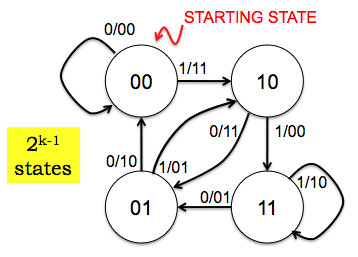
The operation of the encoder may be described as a state machine, as you know (we hope). The figure below is the state transition diagram for a rate 1/2 encoder with K=3 using the following two generator functions:
G0: 111, i.e., p0[n] = (1*x[n] + 1*x[n-1] + 1*x[n-2]) mod 2
G1: 110, i.e., p1[n] = (1*x[n] + 1*x[n-1] + 0*x[n-2]) mod 2
A generator function can described compactly by simply listing its K coefficients as a K-bit binary sequence, or even more compactly (for a human reader) if we construe the K-bit sequence as an integer, e.g., G0: 7 and G1: 6. We will use the latter (integer) representation in this task.
In this diagram the states are labeled with the two previous message bits, x[n-1] and x[n-2], in left-to-right order. The arcs -- representing transitions between states as the encoder completes the processing of the current message bit -- are labeled with x[n]/p0p1.
You can read the transition diagram as follows: "If the encoder is currently in state 11 and if the current message bit is a 0, transmit the parity bits 01 and move to state 01 before processing the next message bit." And so on, for each combination of current states and message bits. The encoder starts in state 00 and you should assume that all the bits before the start were 0.
A stream of parity bits corrupted by additive noise arrives at the receiver. Using the information in these parity bits, the decoder attempts to deduce the actual sequence of states traversed by the encoder and recover the transmitted message. Because of errors, the receiver cannot know exactly what that sequence of states was, but it can determine the most likely sequence using the Viterbi decoding algorithm.
The Viterbi decoder, described in Lecture 9, works by determining a path metric PM[s,n] for each state s and bit time n. Consider all possible encoder state sequences that cause the encoder to be in state s at time n. In hard decision decoding, the most-likely state sequence is the one that produced the parity bit sequence nearest in Hamming distance to the sequence of received parity bits. Each increment in Hamming distance corresponds to a bit error. PM[s,n] records this smallest Hamming distance for each state at the specified time.
The Viterbi algorithm computes PM[…,n] incrementally. Initially
PM[s,0] = 0 if s == starting_state else ∞
The decoding algorithm uses the first set of r parity bits to compute PM[…,1] from PM[…,0]. Then, it uses the next set of r parity bits to compute PM[…,2] from PM[…,1]. It continues in this fashion until it has processed all the received parity bits.
Here are the steps for computing PM[…,n] from PM[…,n-1] using the next set of r parity bits to be processed:
For each state s:
Using the rate 1/2, K=3 encoder above, if s is 10 then, in no particular order, α = 00 and β = 01.
Continuing the example from Step 1: p_α = 11 and p_β = 01.
Continuing the example from Step 2: assuming the received parity bits p_received = 00, then BM_α = hamming(11,00) = 2 and BM_β = hamming(01,00) = 1.
PM_α = PM[α,n-1] + BM_α
PM_β = PM[β,n-1] + BM_β
PM_α is the Hamming distance between the transmitted bits and the parity bits received so far, assuming that we arrive at state s via state α. Similarly, PM_β is the Hamming distance between the transmitted and parity bits received so far, assuming we arrive at state s via state β.
Continuing the example from Step 3: assuming PM[α,n-1]=5 and PM[β,n-1]=3, then PM_α=7 and PM_β=4.
if PM_α <= PM_β:
    PM[s,n] = PM_α
    Predecessor[s,n] = α
else
    PM[s,n] = PM_β
    Predecessor[s,n] = β
Completing the example from step 4: PM[s,n]=4 and Predecessor[s,n]=β.
We can use the following recipe at the receiver to determine the transmitted message:
In this task we'll write the code for some methods of the ViterbiDecoder class. One can make an instance of the class, supplying K and the parity generator functions, and then use the instance to decode messages transmitted by the matching encoder.
The decoder will operate on a sequence of received voltage samples; the choice of which sample to digitize to determine the message bit has already been made, so there's one voltage sample for each bit. The transmitter has sent a 0 Volt sample for a "0" and a 1 Volt sample for a "1", but those nominal voltages have been corrupted by additive Gaussian noise zero mean and non-zero variance. Assume that 0's and 1's appear with equal probability in the transmitted message.
lab4_3.py is the template file for this task (not shown inline here).
You need to write the following functions:
Consider using lab4.hamming(seq1,seq2) which computes the Hamming distance between two binary sequences.
self.predecessor_states
self.expected_parity
self.branch_metric()
The testing code at the end of the template tests your implementation on a few messages and reports whether the decoding was successful or not.
When you're ready to submit your code on-line, enable the call to lab4.checkoff. When submitting, run your task file using python602 because the submission sometimes does not work correctly when run from an integrated development environment.
There are some lab questions associated with this task.
Task 4: Decoding with a soft-decision branch metric (1 point)
Let's change the branch metric to use soft decision decoding, as described in Lecture 9.
The soft metric we'll use is the square of the Euclidean distance between the received vector of dimension r, the number of parity bits produced per message bit, of voltage samples and the expected r-bit vector of parities. Just treat them like a pair of r-dimensional vectors and compute the squared distance.
lab4_4.py is the template file for this task (not shown inline here).
Complete the branch_metric method for the SoftViterbiDecoder class. Note that other than changing the branch metric calculation, the hard decision and soft decision decoders are identical. The code we have provided runs a simple test of your implementation. It also tests whether the branch metrics are as expected.
When you're ready to submit your code on-line, enable the call to lab4.checkoff. When submitting, run your task file using python602 because the submission sometimes does not work correctly when run from an integrated development environment.
There are some lab questions associated with this task.
Task 5: Comparing the performance of error correcting codes (2 points)
In this task we'll run some experiments to measure the probability of a decoding error (i.e., the bit error rate) using the codes you implemented in Tasks 2, 3, and 4 above. There's no additional code for you to write, just some results to analyze. The codes all have rate 1/2:
lab4_5.py is the template file for this task.
Run the code (please be patient, it takes a while; you can do something else while this script does its job). In the end you should see a set of plots of the probability of decoding error (the bit error rate) as a function of the amount of noise on the channel (the x axis is proportional to log(1/noise), tracking the "signal to noise ratio" (SNR) of the channel (see L9 notes for a brief explanation). Larger values of x correspond to lower noise, and a lower error probability for a given coding scheme. Note that the y axis is also on a log scale.
The Task 5 script saves the graph in a PostScript file called lab4data.ps -- during the checkoff interview, you will be asked to show this file to your TA.