Online help is available for both Maple and Matlab:
If you're familiar with Maple, or would rather figure out for yourself what to do (a common feature of MIT students), the worksheet may be downloaded here (you must download Maple worksheets with the right mouse button, or Shift-left button).
athena% add maple
athena% maple&
Now, wait. Maple, like MATLAB, takes a while to load. Also like
MATLAB, the older versions load and run faster (go figure). To load
an older release, the command is
athena% maple -ver 5r3&
(the commands given here will run on the older releases).
If you've downloaded the worksheet, or have your own, you open
these from the File menu item.
The Maple prompt is >. All commands to be executed
must end with a semicolon (;) followed by a return. For
linebreaks within a command, do Shift-return.
All of the commands
given here (in ``keyboard'' or ``teletype''
font) may be copied directly from this page and pasted into your Maple
session (this turns out to be browser-dependent).
First, load the ``Linear Algebra'' package with
with(linalg);
This will give you some idea of what Maple can do, although if you're not familiar with the terms, you might satisfy your curiosity by searching for the commands from the Help window.
Next, define a matrix, starting with, for instance the matrix

(note that the subscripts 1 and 2 are used instead of 0 and s, which were used in lecture).
To enter this as a matrix, the command would be
A1:=matrix([[omega1^2+omega2^2,-omega2^2], [-omega2^2,omega1^2+omega2^2]]);
Remember, if you want a linebreak within a command, it's Shift-return. Note that the labels ``1'' and ``2'' on the frequencies do not show up a subscripts. Deal with it.
To find the eigenvalues of the matrix we've called A1, the command is
eigenvals(A1);
The eigenvalues thus obtained were those found in lecture,
corresponding to the mode where the spring is not strecthed (the
symmetric mode) and the mode where the spring is stretched the same on
both sides (the antisymmetric mode).
The eigenvectors are found with
eigenvects(A1);
What's returned from this command needs explaining. What we get is
two sets, within
(As an aside, try entering the 2×2 identity matrix, called
A4 in the worksheet if you've downloaded, and see what you get.)
You've certainly noticed that if you want both the eigenvalues and the eigenvectors, the eigenvals(A1) command is redundant. It's your choice.
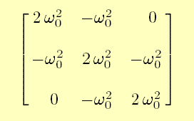
Next, try the 3×3 matrix for the three identical masses coupled by identical springs, with the command
A2:=matrix([[2*omega0^2,-omega0^2,0],[-omega0^2,2*omega0^2,-omega0^2], [0,-omega0^2,2*omega0^2]]);
You should obtain the matrix
 .
.The command
eigenvects(A2);
gives the expected result, except that in two of the eigenvectors, the common factor has not been canceled. This is because Maple is too smart for its own good; if this common factor were zero, which is not precluded on mathematical grounds, the results might be interpreted differently.
One way around this is for us to do the math beforehand, basically factoring out any common term. This also makes it easier to enter the matrix as
A3:=matrix([[2,-1,0],[-1,2,-1],[0,-1,2]]);
and of course the command
eigenvects(A3);
gives the simpler result.
Another useful technique is to extract the desired value and simplify. In this case, the output of the eigenvects(A2) command is a nested set of lists, and the command
r2:=s1[2][3][1][2];
isolates the desired component. From that,
simplify(r2);
gives the simplification.