Using a MEA to Analyze a Dissociated Hippocampal Neural Network
Jonathan Karr (http://web.mit.edu/jkarr/www), Daniel Herman
Presentation: ppt1 ppt2 | pdf | pdf (six slides per page) | ram
The interconnections formed by neurons in dissociated culture have remained elusive. We have proposed and begun to develop the methods necessary to extract the network architecture of a dissociated culture of hippocampal neurons. Using data obtained from multi-electrode array (MEA) studies of dissociated hippocampal cultures, we have demonstrated the use of template spike convolution and cluster cutting to identify individual neurons. To analyze the broad scale network connections we have developed a convolution method and validated it using a toy network. Ultimately, these protocols will yield a method for modeling dissociated networks and facilitate studies of neural network formation, properties, and interfacing.
Here we use a multi-electrode array (MEA) to analyze a hippocampal network. Our goal is to develop a map of the neural network, diagramming the connections between neurons. The multi-electrode array approach has many advantages over the patch clamping method including the ability to monitor many neurons at once, the ability to monitors neurons over an extended period of time, and greater ease of use. Multi-electrode arrays however, do not monitor individual neurons. Each electrode in the array is capable of detecting the spike activity of many neurons2. Below we discuss a framework for connecting the electrode level provided by the array to the level of individual neurons.
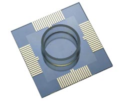
The particular multi-electrode array used is the Panasonic MED64. The array has 64 electrodes, arranged in a 8 x 8 grid as diagrammed below. Each electrode is 50µm x 50µm; adjacent electrodes are spaced by 150µm1. The largest distance between two electrode is 1.7mm which is on the order of a typical hippocampal neuron projection. Thus neurons located at any two electrodes could be connected. The analysis we present below will take this fact into consideration.
Figure 1. MED64 Array1
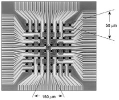
Figure 2. MED64 Array1
|
1 |
2 |
3 |
4 |
5 |
6 |
7 |
8 |
|
9 |
10 |
11 |
12 |
13 |
14 |
15 |
16 |
|
17 |
18 |
19 |
20 |
21 |
22 |
23 |
24 |
|
25 |
26 |
27 |
28 |
29 |
30 |
31 |
32 |
|
33 |
34 |
35 |
36 |
37 |
38 |
39 |
40 |
|
41 |
42 |
43 |
44 |
45 |
46 |
47 |
48 |
|
49 |
50 |
51 |
52 |
53 |
54 |
55 |
56 |
|
57 |
58 |
59 |
60 |
61 |
62 |
63 |
64 |
Figure 3. Electrode layout
As stated previously, our goal is to access the connectivity of neurons in a neural network. We do so by iteratively stimulating each electrode and then taking correlations between the stimulated electrode and every other electrode. The underlying assumption here is that random neural spiking is negligible compared to the spiking induced by stimulation. Thus stimulation yields a starting point from which to analyze the network; stimulation allows to attribute all neural activity to the spiking of the stimulated neurons (those neurons located near the stimulating electrode). A more precise approach might perform the same analysis which would yield a matrix of connections and then subtract from that matrix the result of applying the analysis to the network in the absence of stimulation.
The resulting matrix of connections contains both a representation of connection strength and delay. Connection strength between electrodes is determined by the maximum correlation value. Connection strength is stored as the real part of each entry. The time delay corresponding to this maximum correlation is taken as a measure of distance between electrodes (i.e. how many electrodes separate two given electrodes if the two given electrodes are indirectly connected through other electrodes). Delay is stored as the imaginary part of each entry. We then compute a graphical display of the neuronal connections.
Matlab code
Before proceeding to analyze hippocampal data using the method outlined above we apply the method to a computer generated network, which henceforth will be referred to as the ‘toy network.’ The network we used consisted of nine neurons connected in a specified fashion shown below. We then generated nine sets of spikes corresponding to the stimulation of each of the neurons using the set of specified connections. The model makes the following assumptions: 1) Signal transduction delay (time required for a signal to propagate across the length of a neuron) is negligible in comparison to synaptic delay and can thus be ignored. 2) Any pair of neurons can be connected. This assumption was justified in the introduction. The model includes parameters for refractory period length, synaptic delay, and connection strength.
Next we analyzed the spikes and according to the method outlined in the previous section. Below are two graphs of the connections we found in our simulated network. The derived connections are almost identical to their specified values, in particular the first order connections (marked in red) are the same as the first order connections programmed into the network. The derived graphs also show the effect of higher order (indirect) connections; these connections are marked in other colors which range from red (least delay) to black (most delay).
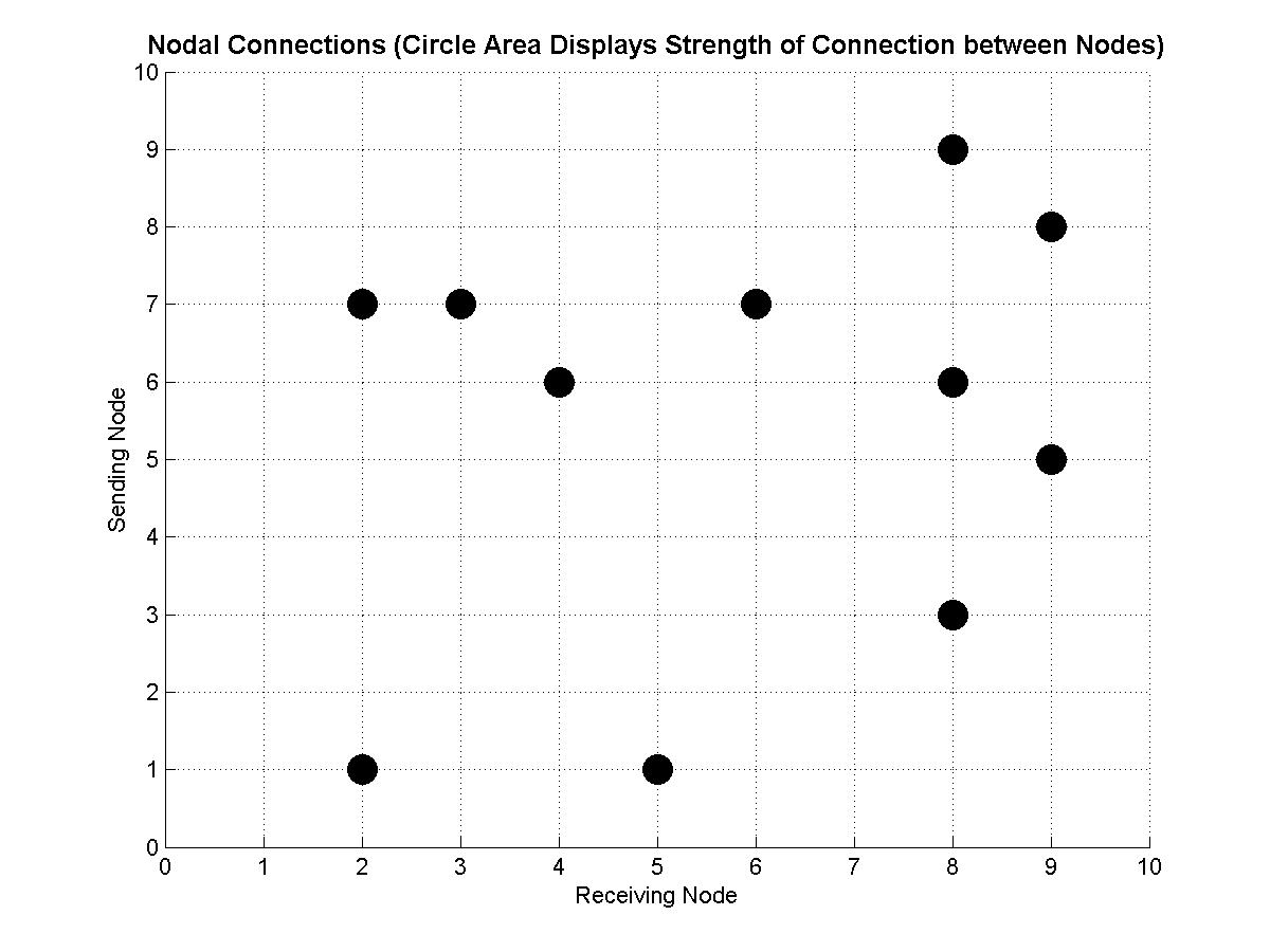
Figure 4. Representation of the first order connections in the toy network. Connection strength is represented by shaded area.
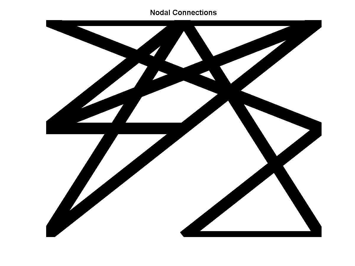
Figure 5. Map of the electrons in the toy network. Connection strength is represented by line width.
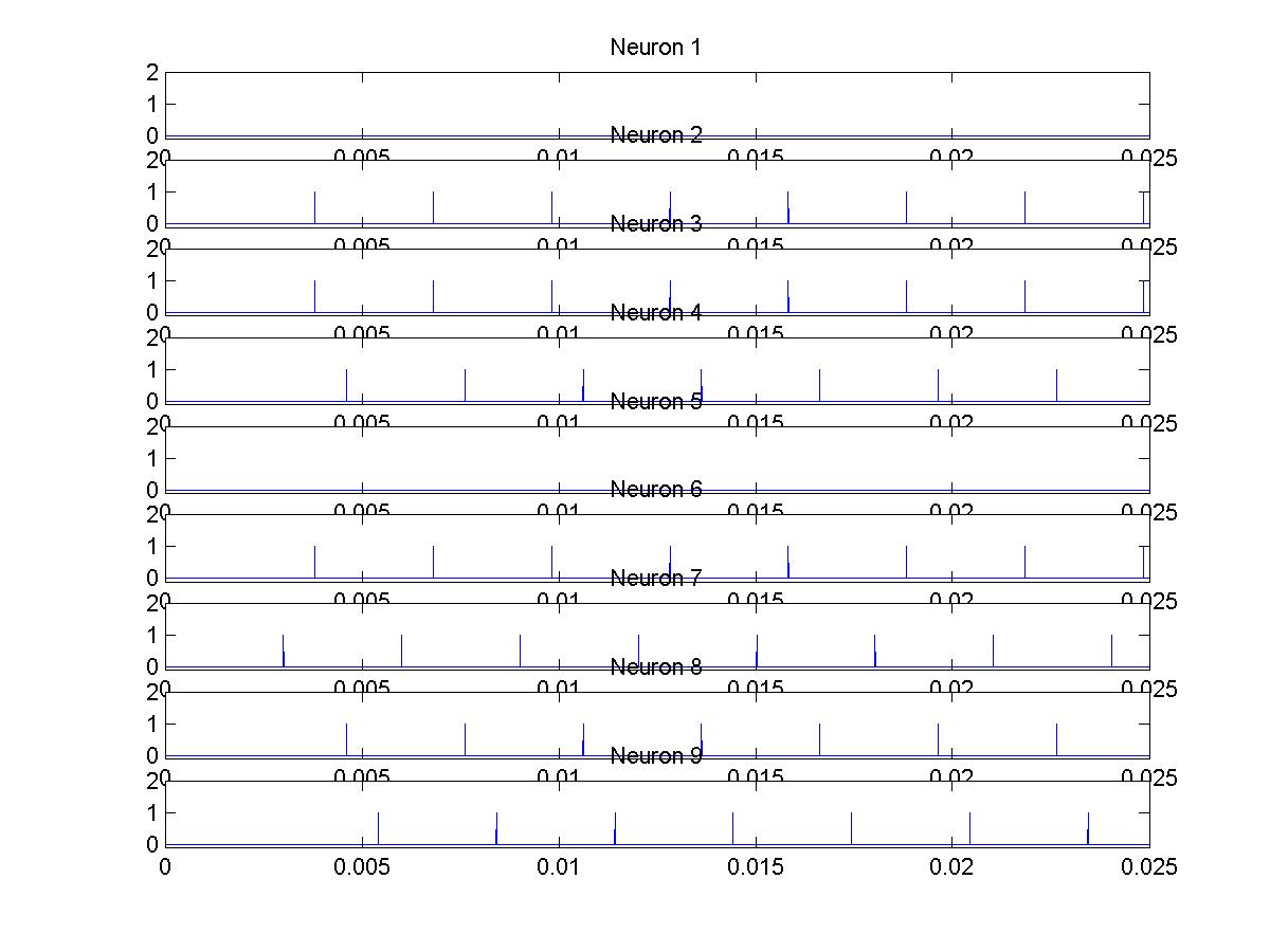
Figure 6. Spikes for each of the nine neurons in the toy network when neuron 7 is stimulated.
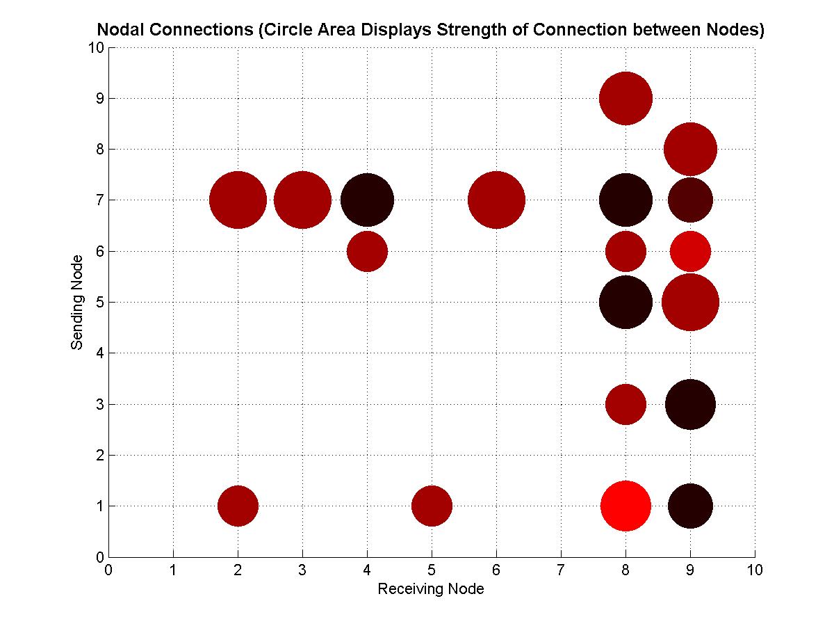
Figure 7. Representation of the connections (found by analysis) in the toy network. Connection strength is represented by shaded area. Time delay is represented by color. Red indicates a short delay. Black indicates a longer delay.

Figure 8. Map of the electrons in the toy network as determined by the analysis. Connection strength is represented by line width. Time delay is represented by color. Red indicates a short delay. Black indicates a longer delay.
Toy Network 'Data'
toynetwork_connectionsfound.mat
Matlab code
Here we apply the network analysis method outlined above to a hippocampal culture. The first in analyzing the hippocampal culture is to extract spikes from the recorded data6,7. For each electrode this consists of:
1) Detrending the data to remove any linear trends in the data. This is accomplished using the MATLAB command detrend.
2) Removing the very large sixty hertz osicallation as well as other frequencies with unusually large components. This was done by computing the fourier transform of the recorded data and zeroing out any frequency with an amplitude greater than the threshold value. At this step we also zeroed out frequencies above 5000Hz and below 500Hz as such frequencies do not correspond to the spiking of neurons. Finally we compute the inverse fourier transform to return to the time-space.
3) Determining the location of spikes. We accomplished this by applying a threshold equal to a multiple of the standard deviation of the signal. The locations of the spikes were stored in a separate matrix.
The analysis method can then be applied to the extracted spikes to determine the connectivity of the 64 electrodes. It should be noted that the analysis takes a significant amount of time as it requires n(n-1) correlations, where n is the number of electrodes. For example if you have data from stimulating all 64 electrodes, this method prescribes 4032 correlations, each of which requires maxdelay*m2, where m is the number of data points and maxdelay is the recursion limit for computing higher order connections. We however only had data from the stimulation of 12 electrodes; thus 756 correlations were required which required approximately 4.35456 x 10¹⁴ multiplications. Below the results of the analysis are presented in two graphical forms.
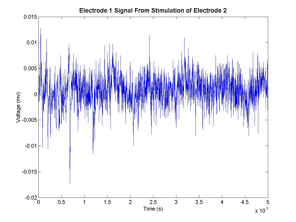
Figure 9. Representative unfiltered signal. Near t=0 there is a very prominent transient behavior due to the stimulation of the network. 50 ms later the network has settled into its steady-state and all transient behavior is absent.
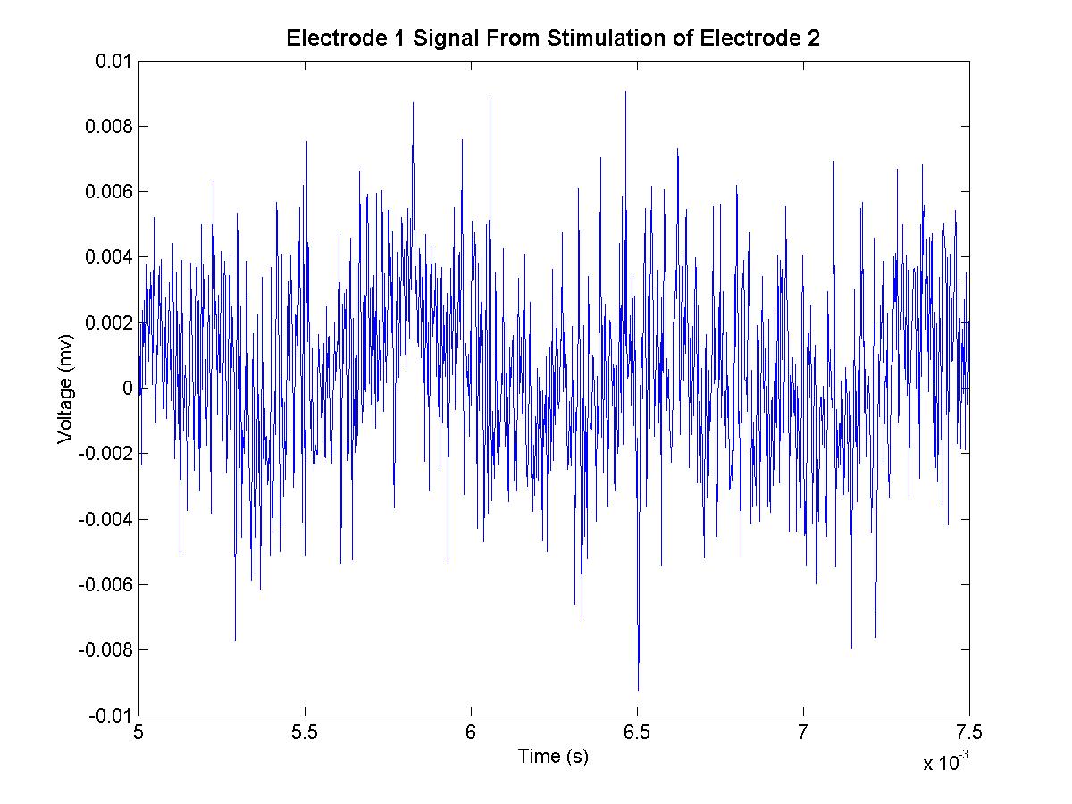
Figure 10. Representative unfiltered signal after the initial transient behavior has died out. The unfiltered signal has a very prominent 60Hz oscillation.
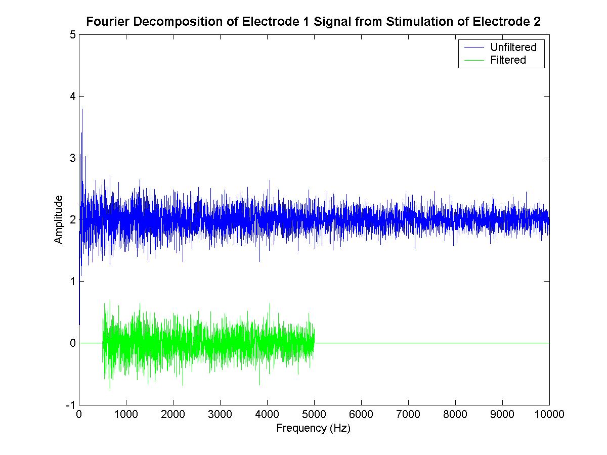
Figure 11. Power Spectrum of a representative signal before and after filtering.
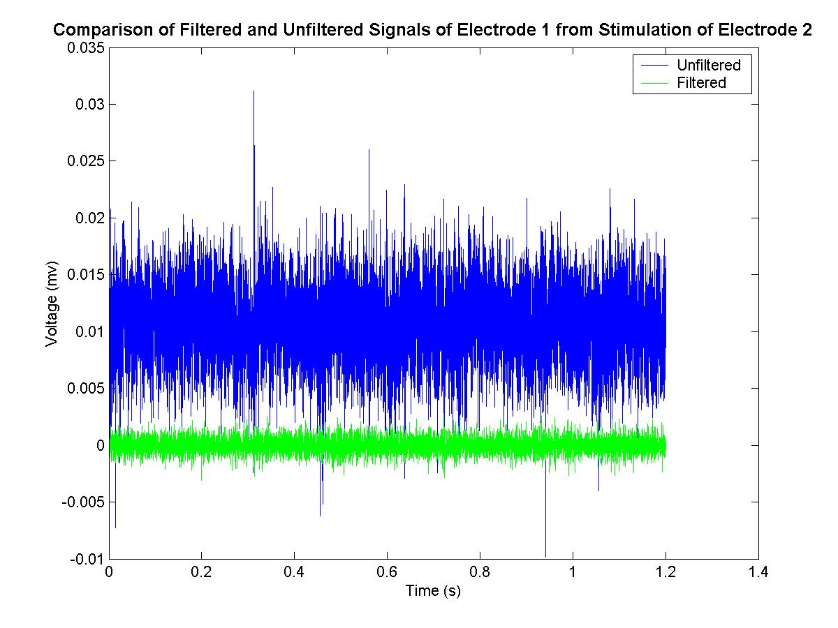
Figure 12. Comparison of representative filtered and unfiltered signals. The most striking change is the absence of the 60Hz oscillation.
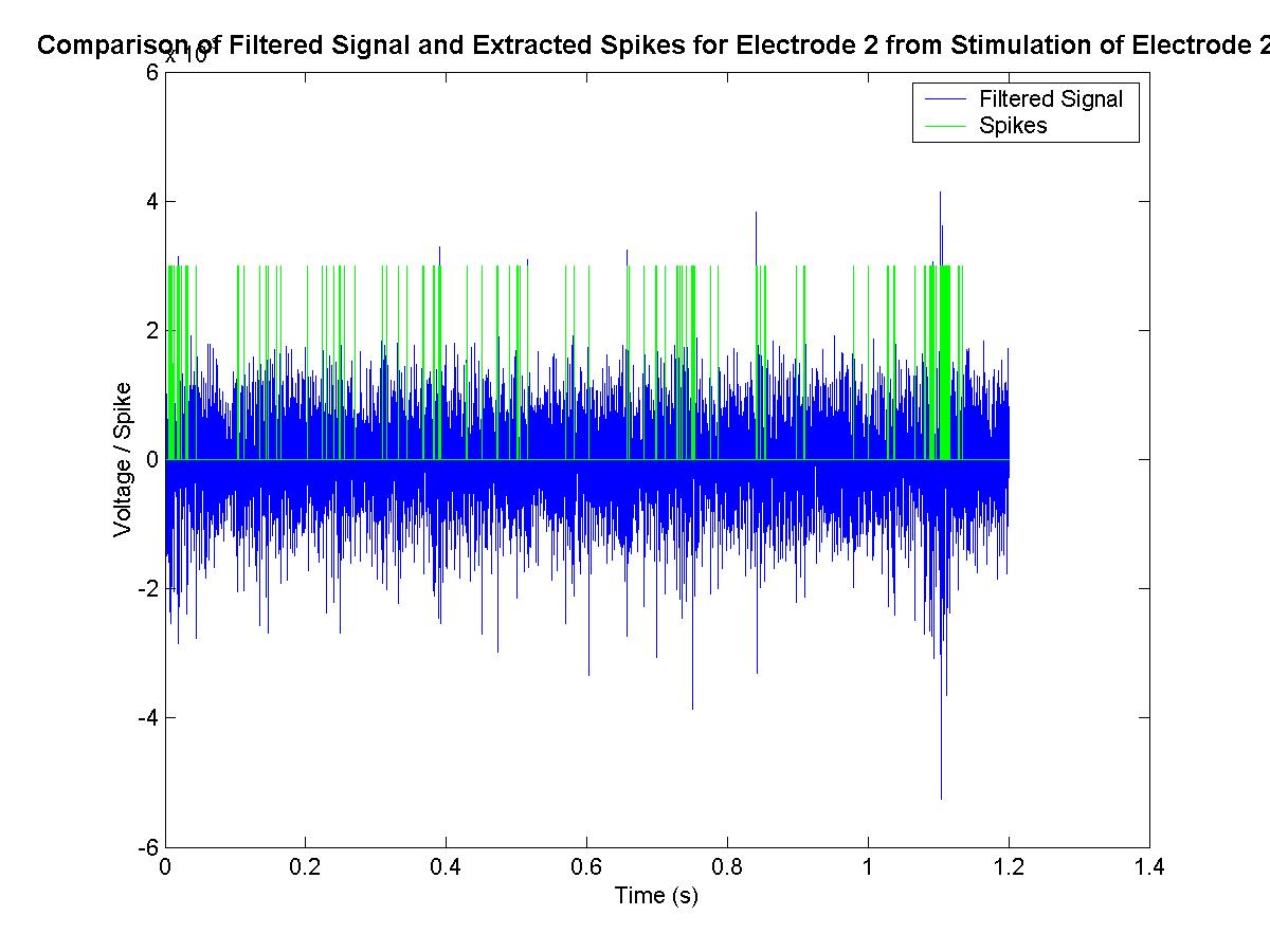
Figure 13. Comparison of filtered signal and extracted spikes.
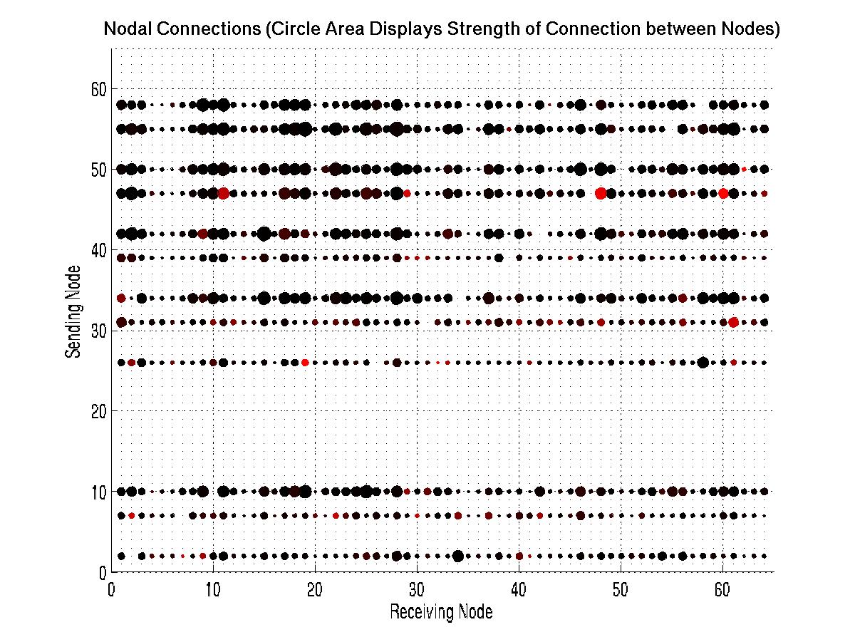
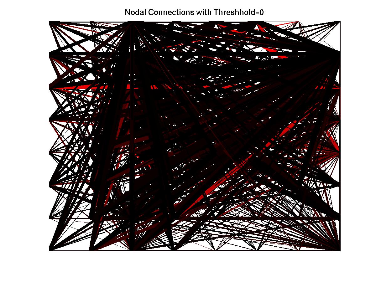
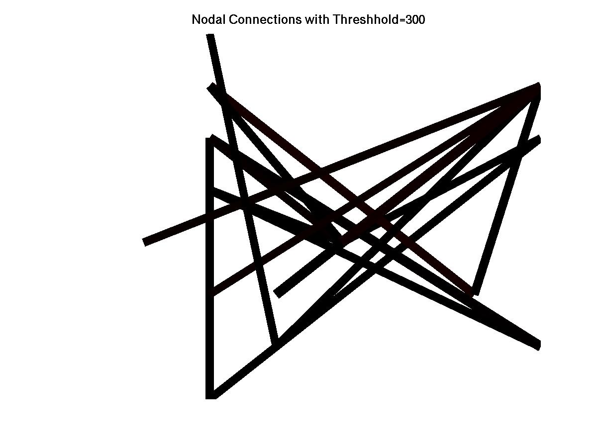
Figure 14. Representation of the connections in the hippocampal network. Connections strength is represented by area. Time delay is represented by color where red indicates a short delay and black indicates a long delay.
 |
 |
 |
 |
 |
 |
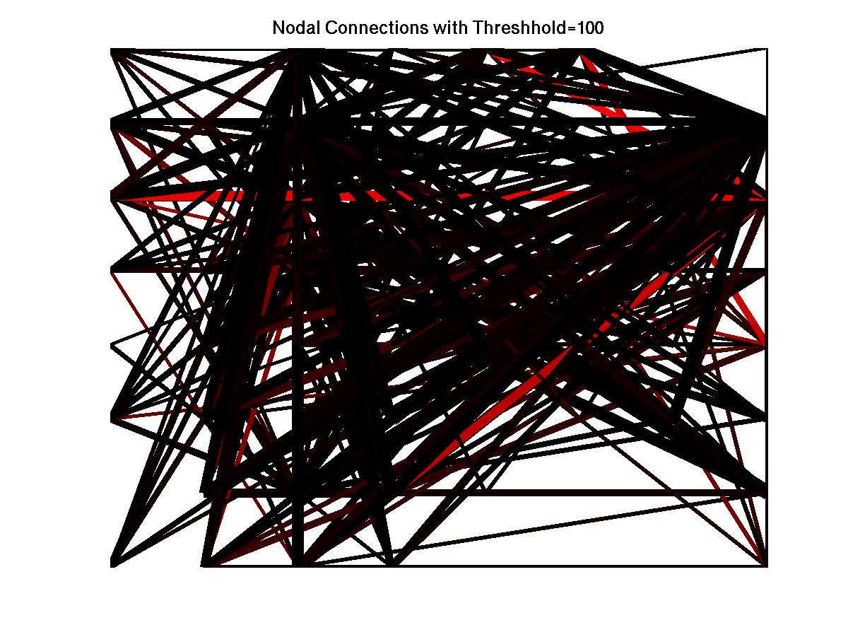
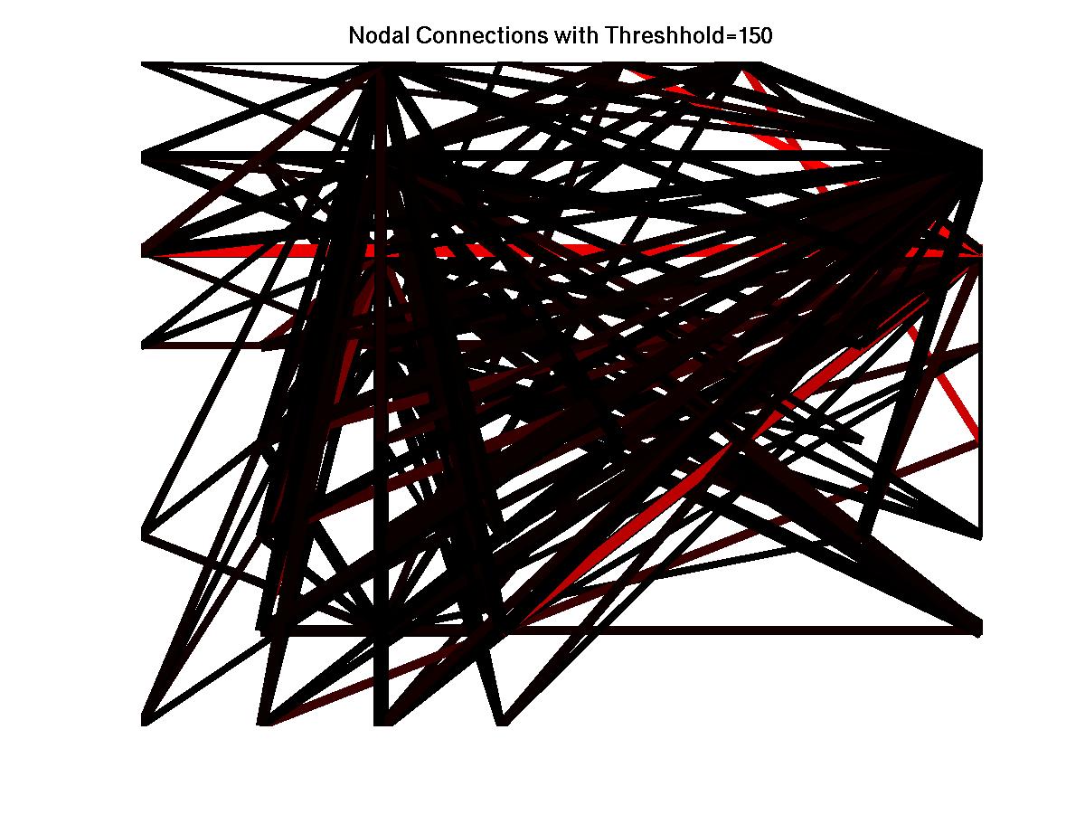
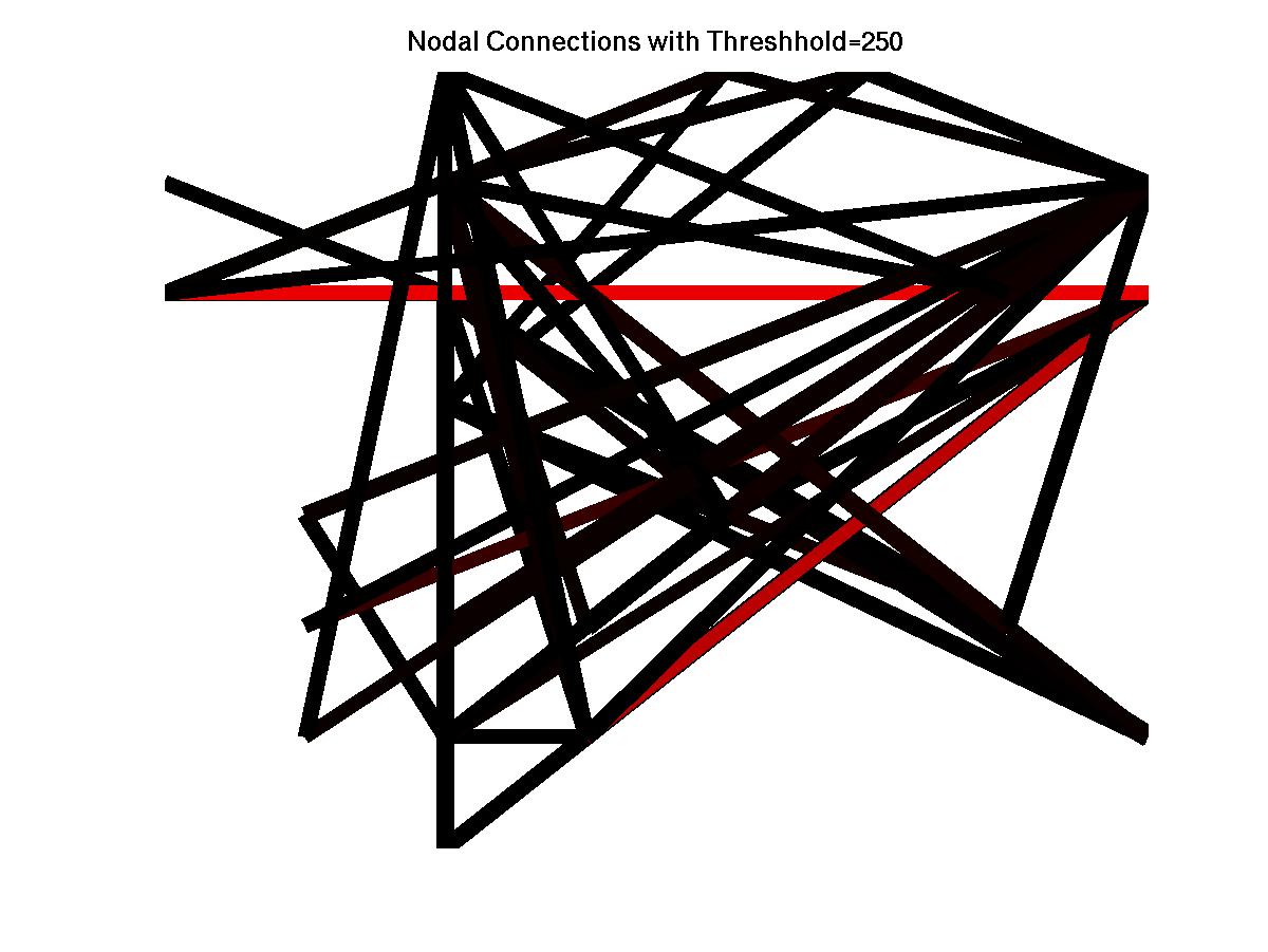
Figure 15. Map of the hippocampal network at different connection threshold values. Connection strength is represented by line width. Time delay is represented by color where red indicates a short delay and black indicates a long delay.
Hippocampal Data (Extracted Spikes)
Matlab code
plots.m (creates graphics in this section)
VI. Spike Sorting By Convolution
The preceding analysis of the hippocampal network worked at the level of electrodes. Using the analysis method discussed in part II we were able to generate a diagram of the connections between the sixty four electrodes of the recording array. Here our goal is to perform the same analysis, but at the level of individual neurons rather than electrodes. We will do this by separating out the spikes of individual neurons from the signal of a given electrode. In doing so we will take advantage of the fact that the spikes of one neuron can differ in shape from a second neuron.
For such a separation to be possible it is required that each neuron located at a given electrode have a different spike shape. Here we determine the minimum number of different shapes needed to guarantee (probability of .9) that each neuron located at a given electrode will have a different shape. We assume that 1) each spike shape is equally likely, 2) spike shapes are randomly distributed, and 3) the maximum number of neurons the are located at a given electrode is 2. We want to solve the following equation for n:
![]()
By this crude calculation we see that we need ten shapes for such a separation to be possible.
The method we propose for separating the spikes of individual neurons from the signal of a given electrode is to convolve the filtered signal of each electrode with template spikes. The template spikes used will be a representative spike for each of the ten different types of neurons (classified by spike shape). Convolved signals with less than a minimum number of spikes will be discarded. The remaining convolved signals will become the neurons located at a given electrode3,4,5. The second part of the analysis where we before computed correlations between the stimulated electrode and all other electrodes will remain the same with the exception that individual neurons will be used in place of electrodes. A side note, were the electrodes spaced closer together it might also be possible to determine the physical location of individual neurons. To make such a calculation one could look at the contributions of an individual to neuron at neighboring electrodes. One could find these contributions by convolving the representative spikes with these neighboring electrodes and then comparing the times of observed spikes. If at multiple electrodes one observes spikes of the same shape at the same time or displaced by some delay one could calculate the position of the neuron with some additional assumptions about the cause of the delay (i.e. resistance due to the extracellular medium). Again such calculations would require the assumption that there is at most one type of neuron in a given spatial neighborhood.
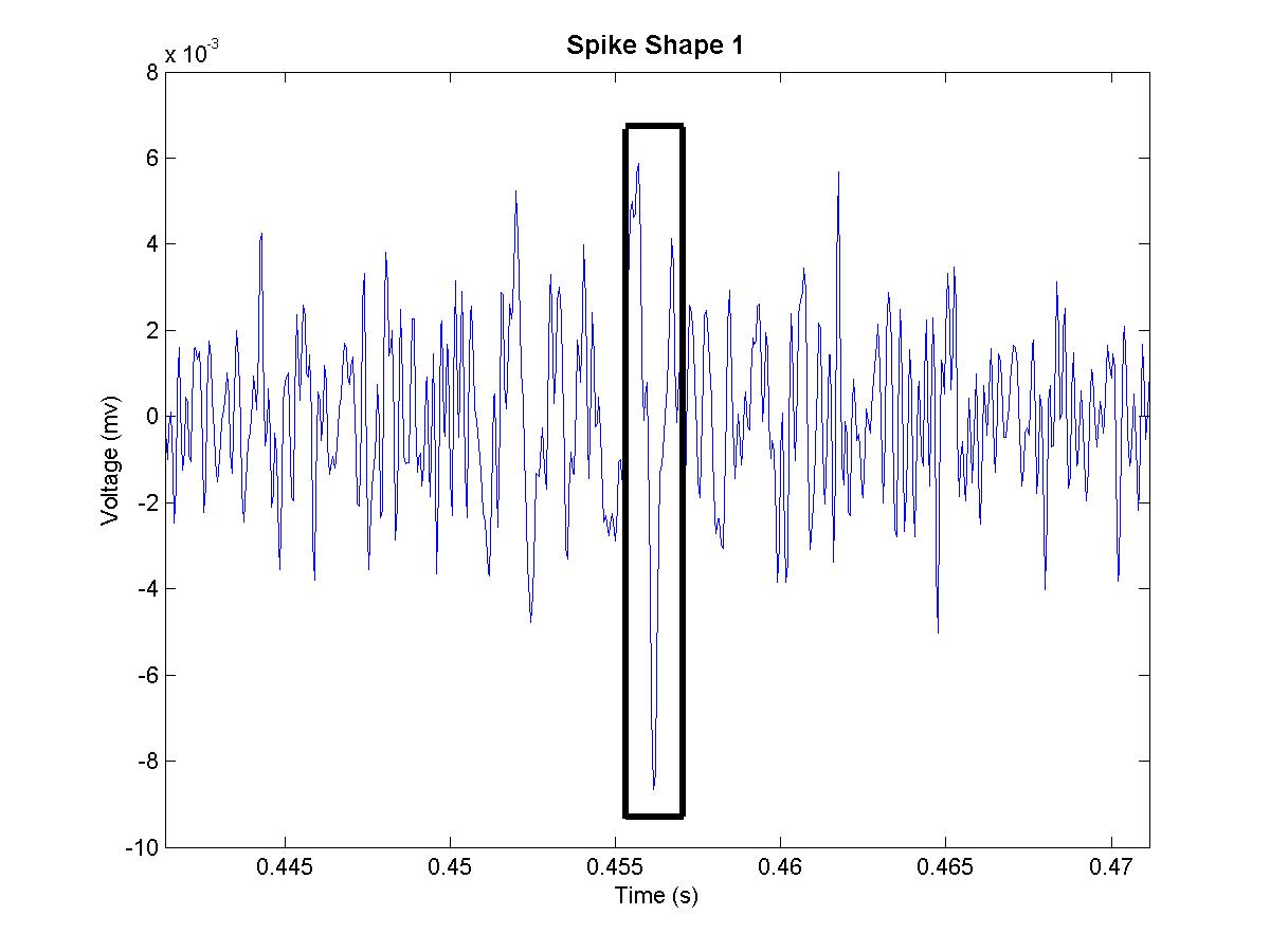
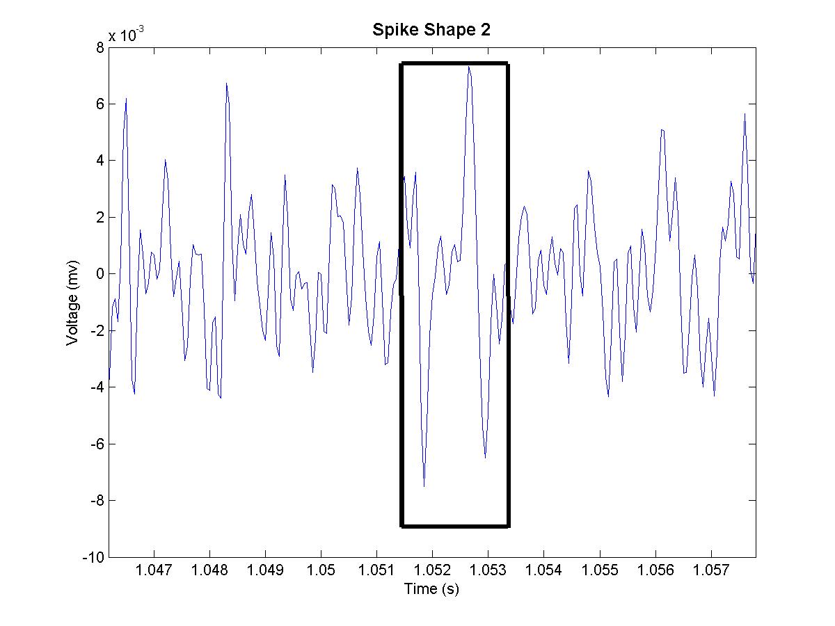
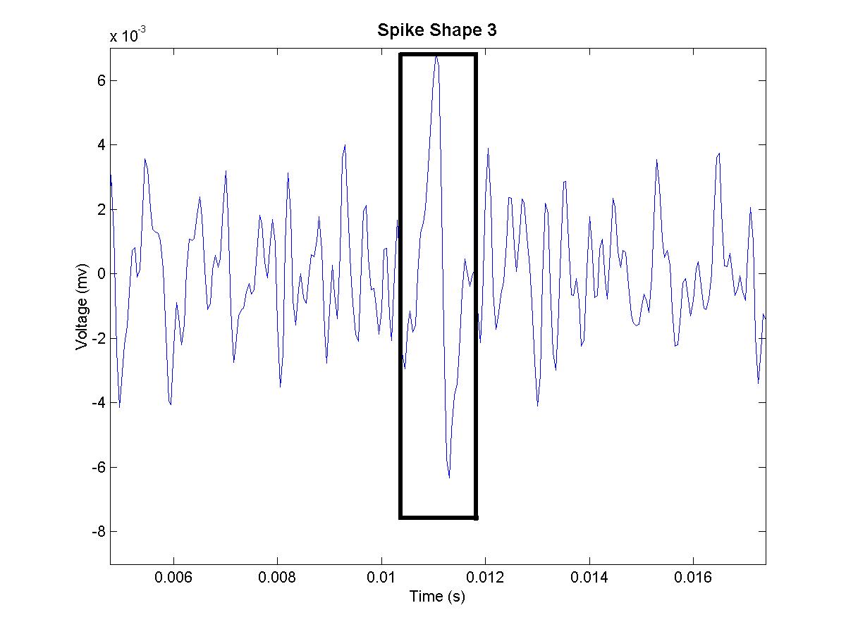
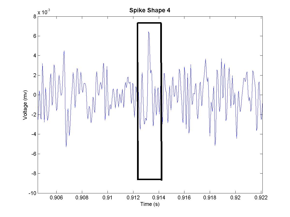
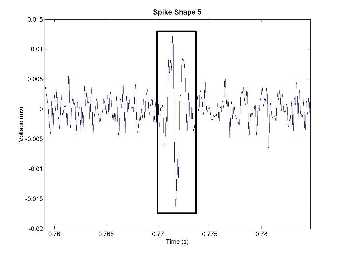
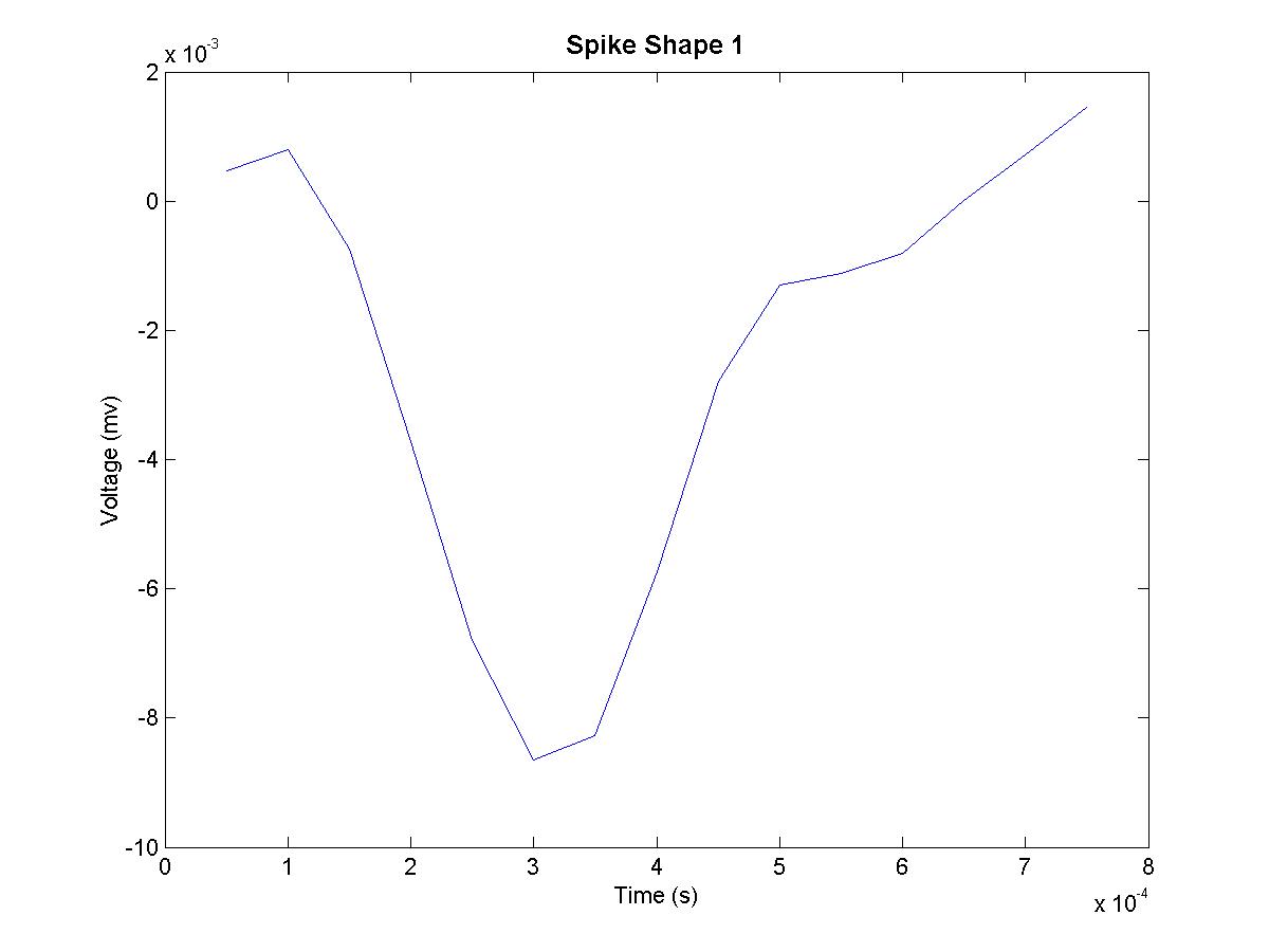
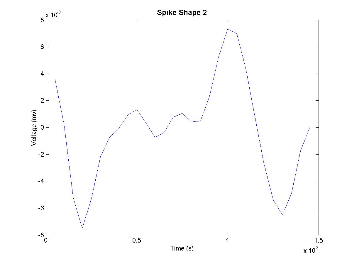
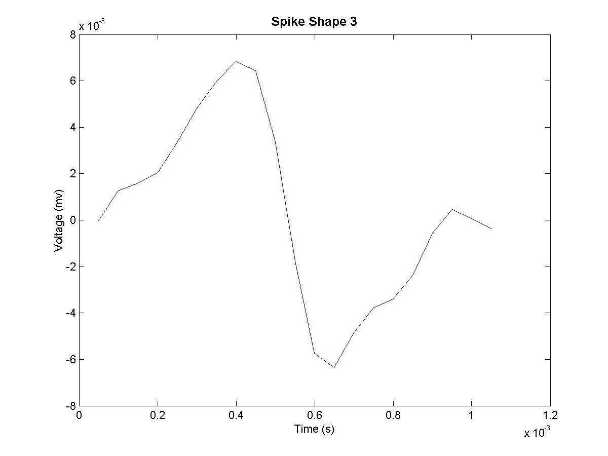
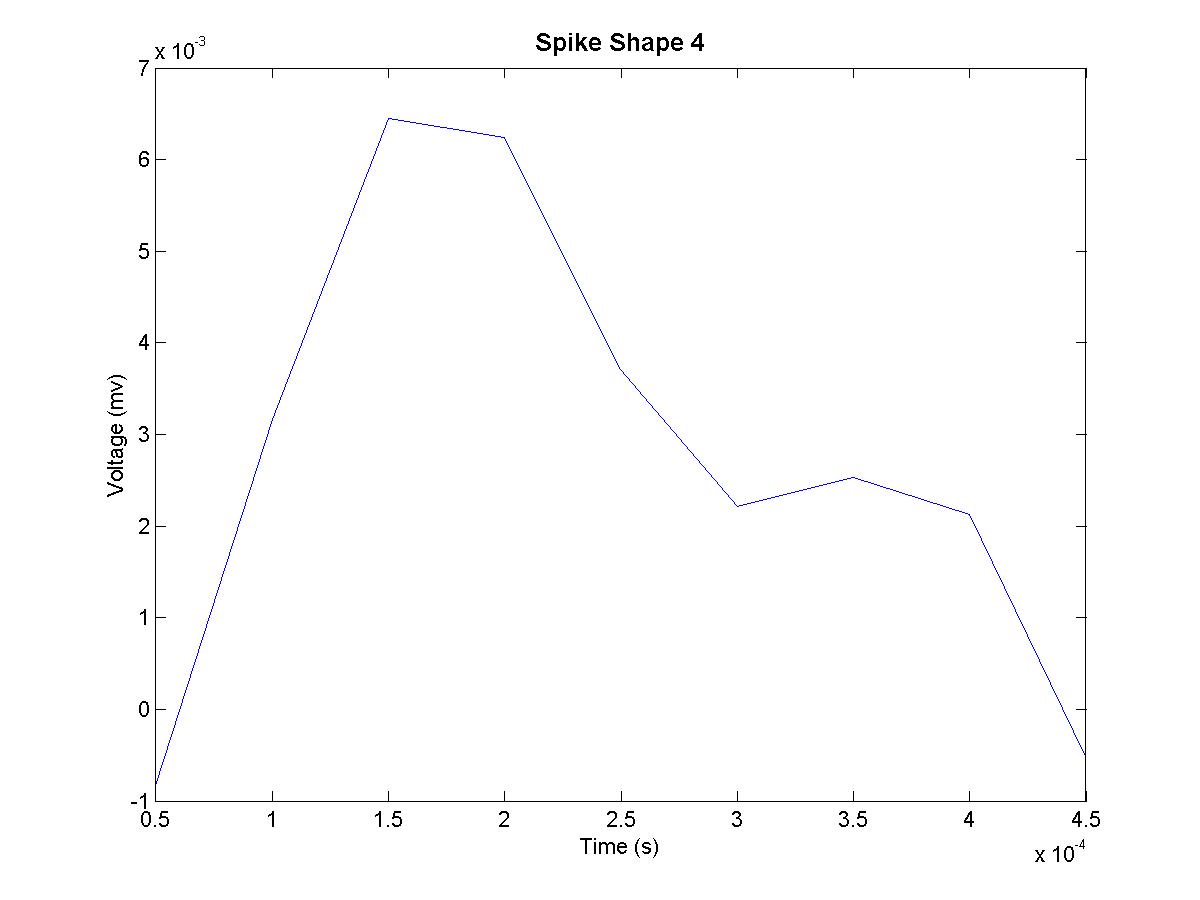
The task then is to identify ten distinct spike shapes or if that is not possible to cultivate neuronal cell lines which have at least ten different spike shapes. Below are different spike shapes observed in the same hippocampal data that was filtered and analyzed in the previous section.
 |
 |
 |
 |
 |
 |
 |
 |
 |
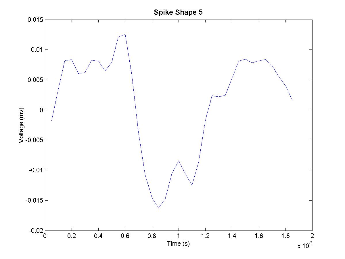 |
Figure 16. Five different observed spike shapes in electrodes 60-64.
 |
 |
 |
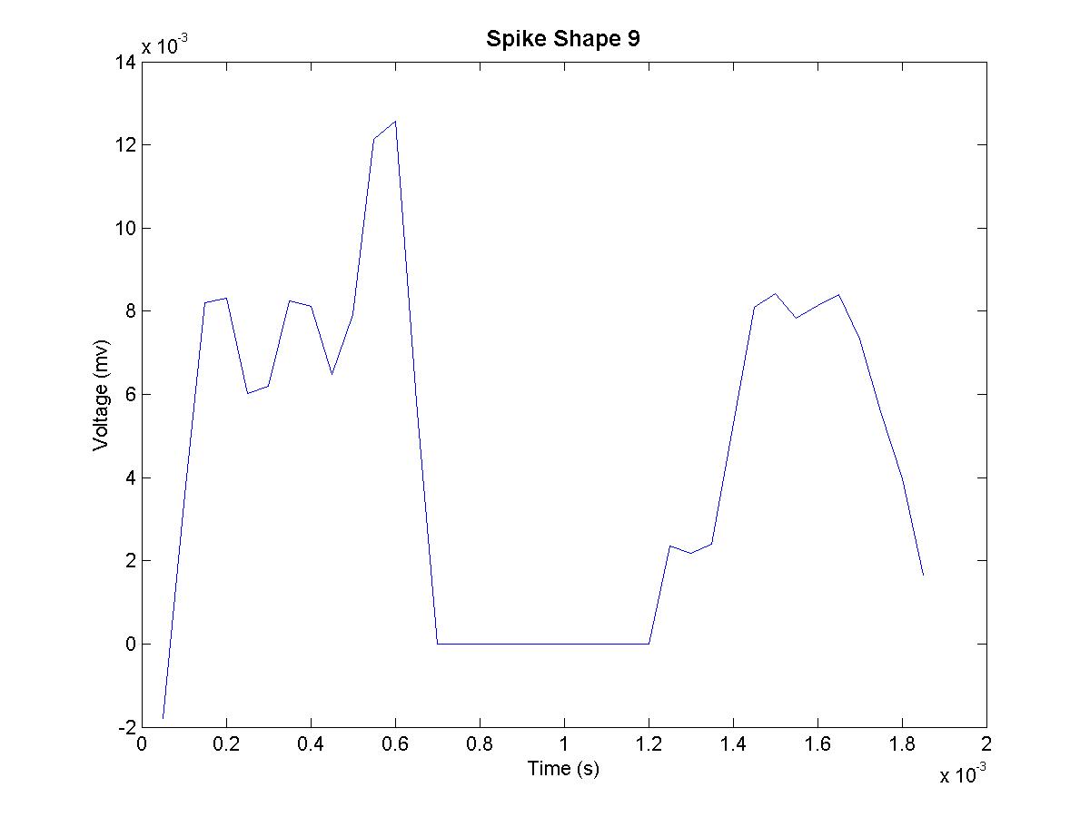 |
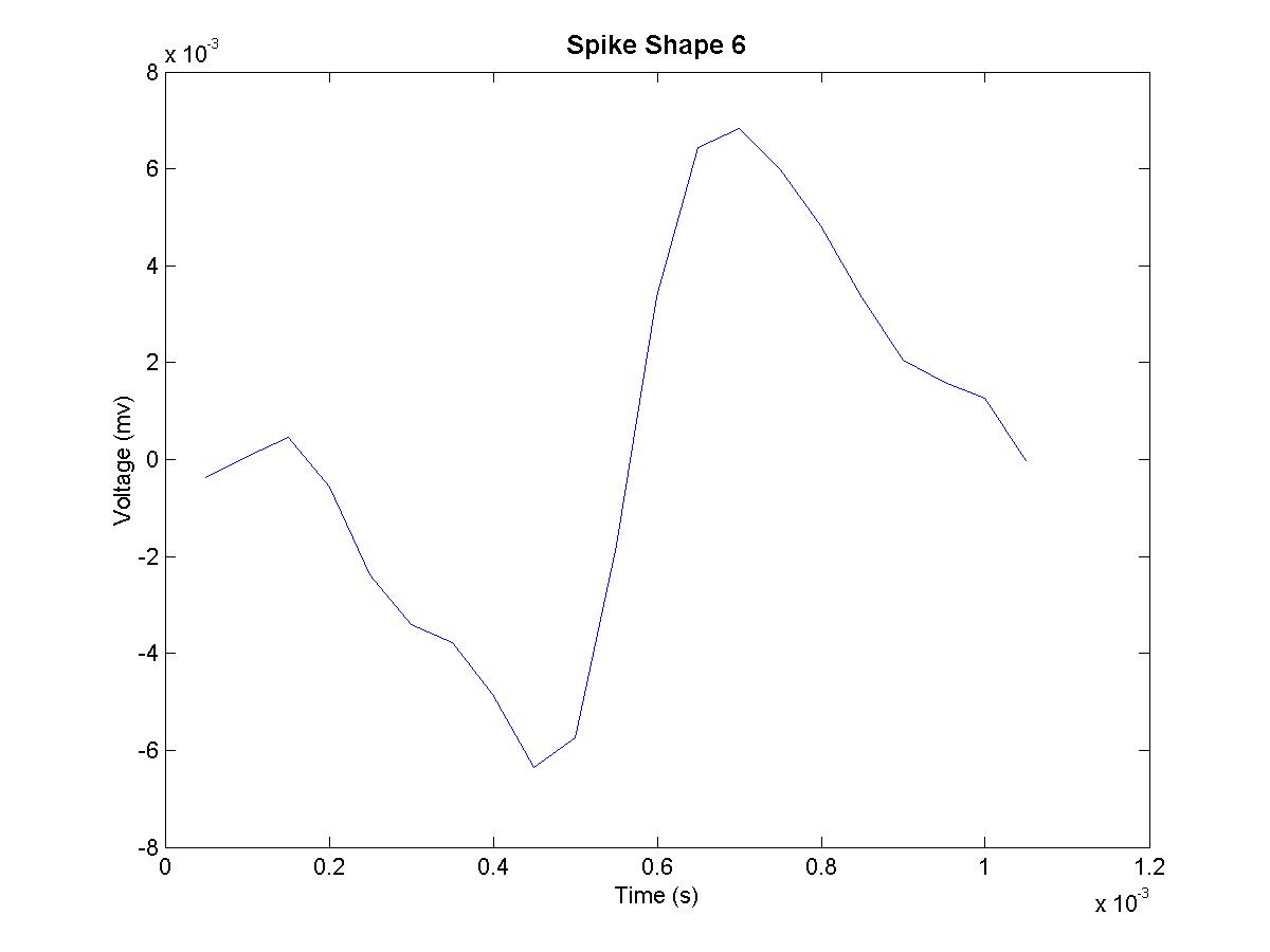
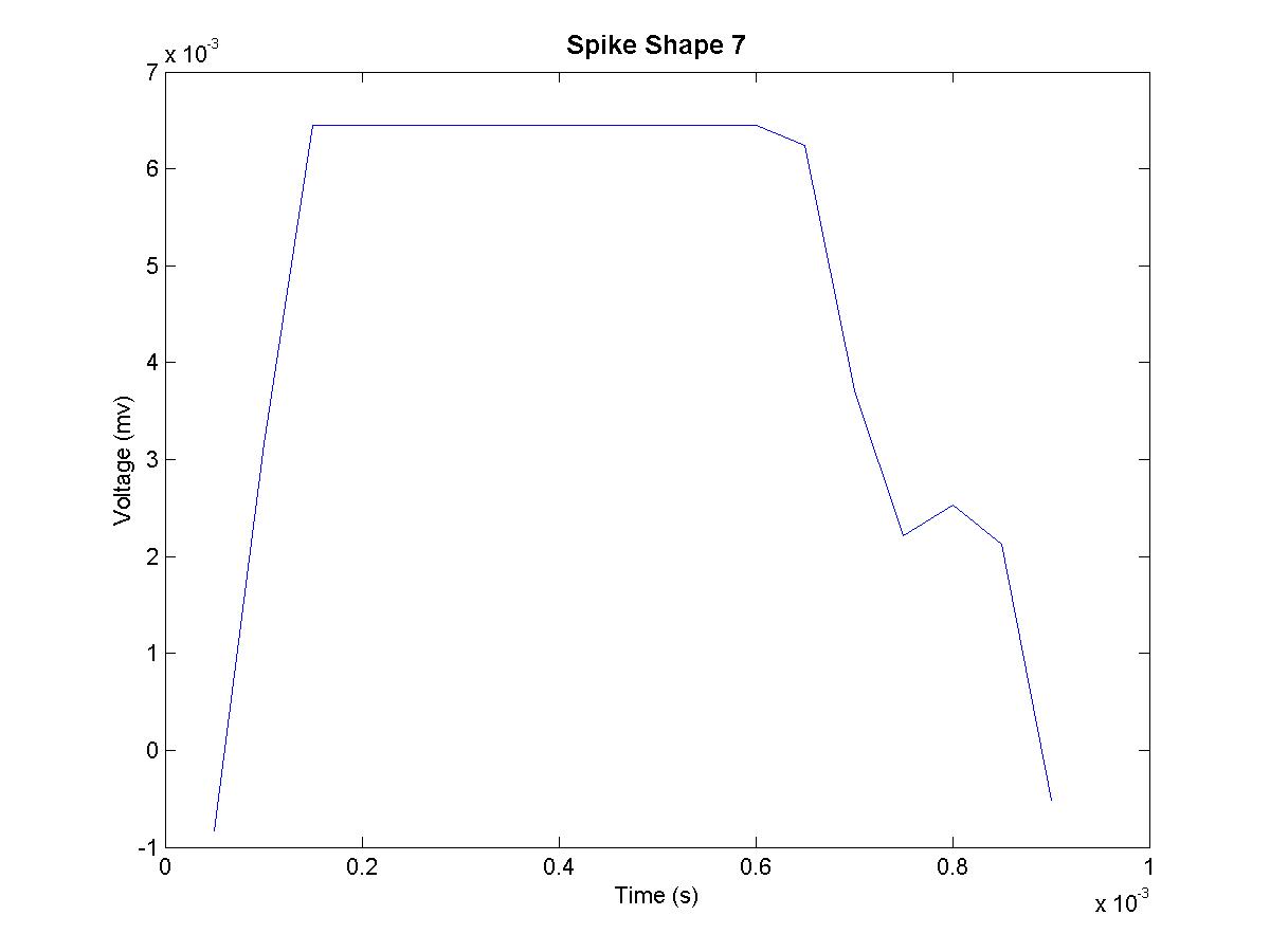
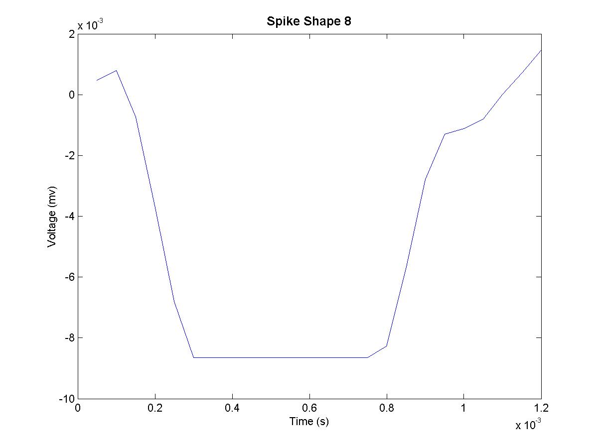
 |
Figure 17. Five additional shapes. These shapes were not observed upon visual inspection; rather they are proposed shapes. Shape 6 is the reverse of shape 3. Shape 7 is shape 4 with a longer plateau. Shape 8 is shape 1with a longer minimum. Shape 9 is 5 with the minimum set to zero. Shape 10 is the negative of shape 9.
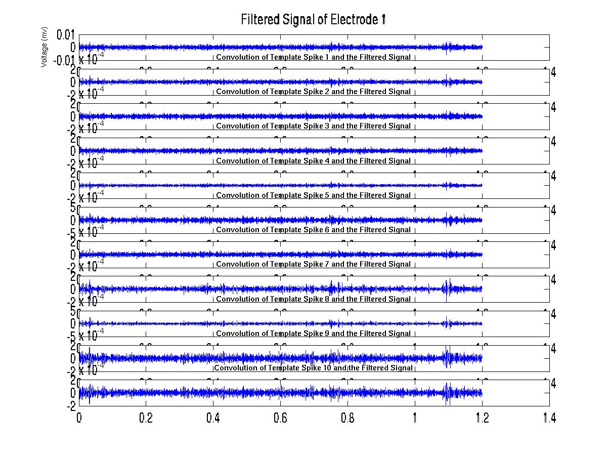
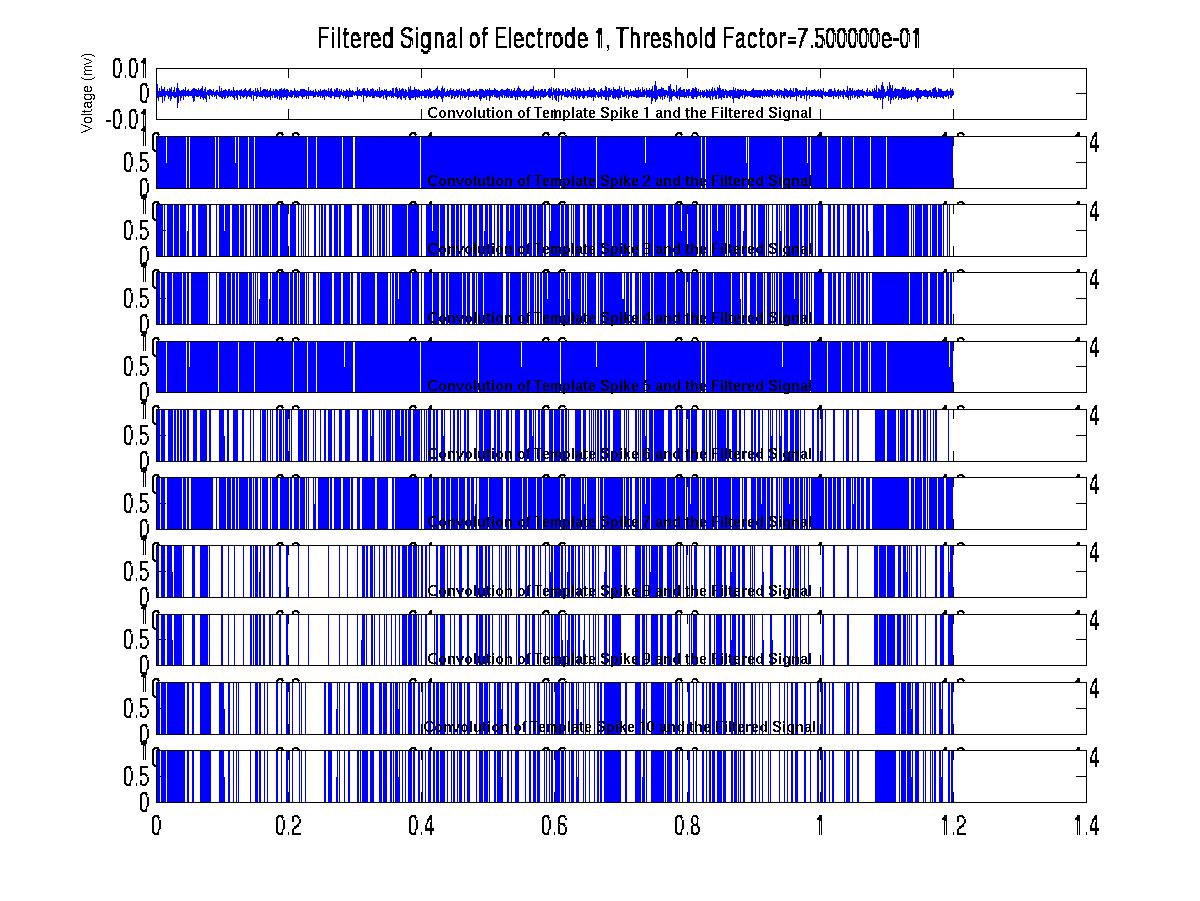
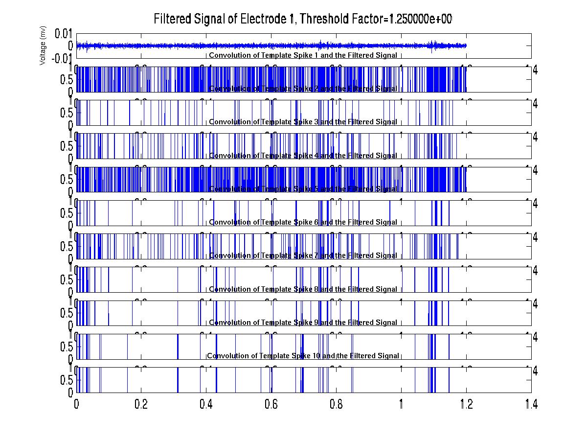
Figure 18. Result of convolving the filtered signal from electrode 1 when electrode 2 was stimulated.
 |
 |
 |
Figure 19. Result of applying thresholds to the convolution of electrode 1 with the different spike shapes. The result shows evidence of neurons of shape 1 and 4 at electrode 1.
Template Spikes
template_spikes.m (creates the template spikes)
Matlab Code
my_analyzeremap2_individualneurons.m
VII. Spike Sorting By Cluster Cutting
An alternative technique for detecting individual neurons from the signal of one electron is cluster cutting6,8,9. In this technique spikes are categorized according to various parameters such as spike height and spike width and then spikes are separated by on the parameters. The advantage of this technique is that it requires less information; this method needs only a small number of parameters rather than template spikes. While this method permits cleaner separation after extensive training and has the ability to detect simultaneous spikes, it comes at the price of more challenging classification and computation. Moreover, cluster cutting method is only possible if there are distinct groups in the multi-dimensional space characterized by the various features.
For this analysis data from electrode 2 following stimulation of electrode 2 was filtered and spikes were extracted (Fig. 20)
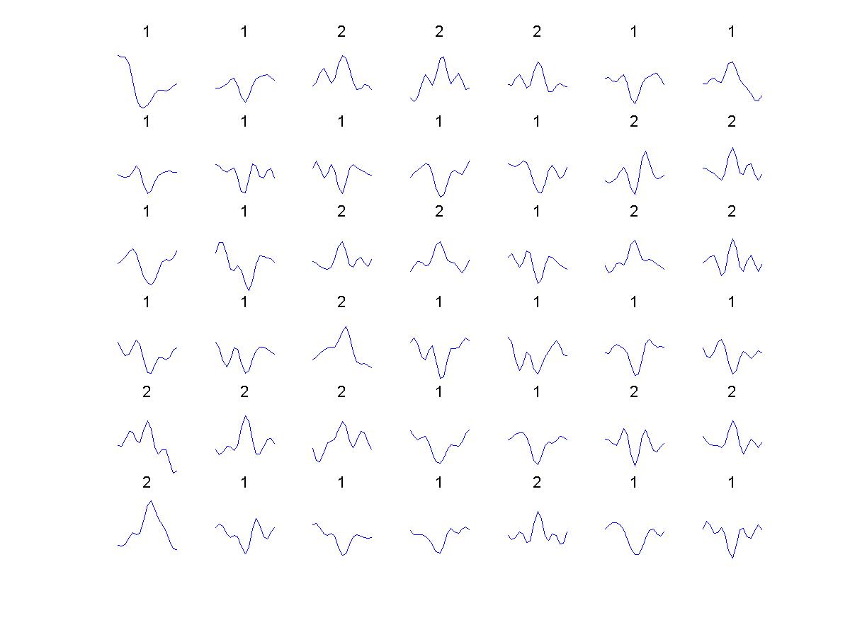
Figure 20. An array of spikes found identified in remap2pin02 classified as type 1 or 2 by inspection; Width = 0.85 msec.
Each spike was analyzed for (1) height of maximum peak, (2) height difference between maximum and second maximum peak, (3) sum of maximum positive and maximum negative peak, (4) time between maximum positive and maximum negative peaks, and (5) maximum width of a departure from the reference voltage.
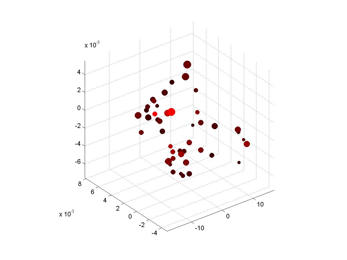
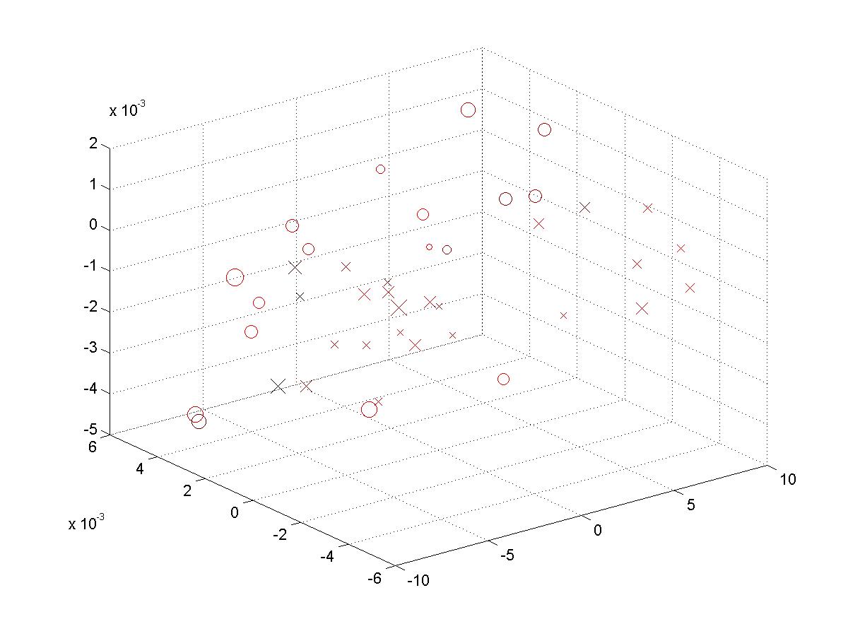
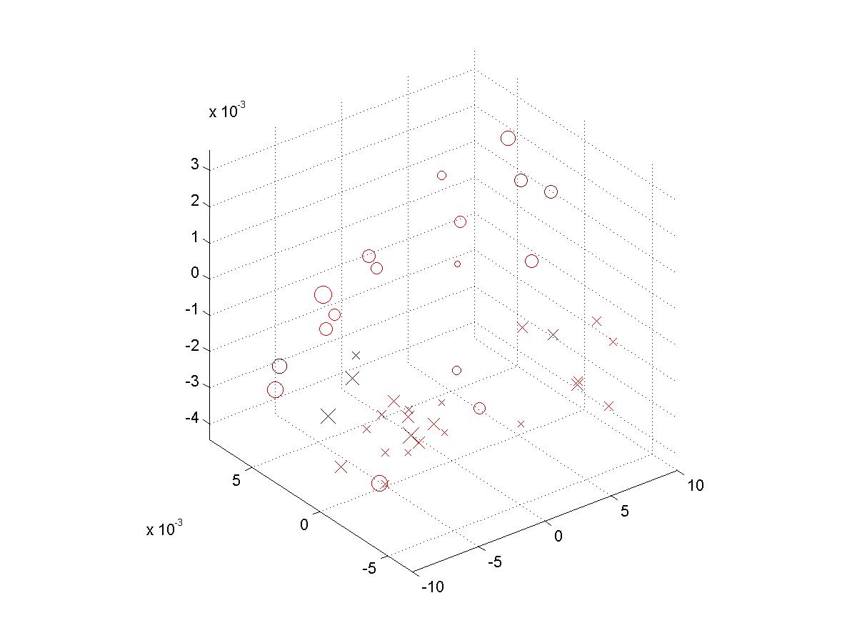
Figure 21. A 3d plot of spikes in remap2pin02 trial 53. X-axis represents time between max positive and max negative peaks, Y-axis represents the sum of the maximum positive and negative peaks, Z-axis represents the voltage difference between the maximum and second maximum peaks, the size of the dots represents maximum width of a departure from the baseline voltage, and the color represents the height of the maximum peak.
  |
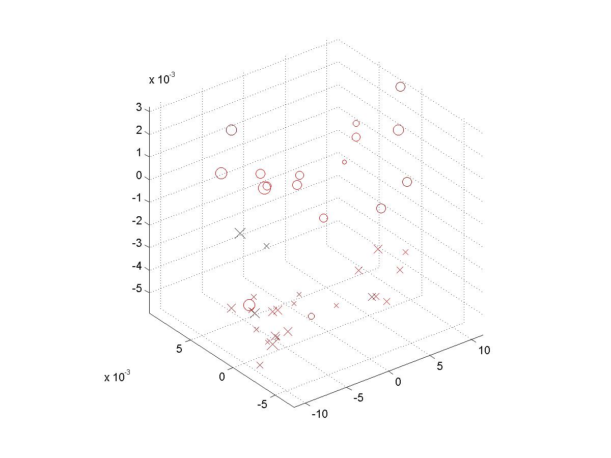 |
Figure 22. Three different views of a 3d plot of spikes in a remap2pin02 trial 53 as in Fig. 21, where X's represent type 1 spikes and O's represent type 2 spikes.

Figure 23. Plot of spikes in same trial. Sum of max positive and negative peaks vs. Time between polarizations
In this case, although they are too far apart, there is a good separation seen in each of the plots in figures 22 and 23. In this case, the sum of the max positive and negative peaks is almost enough to separate the two classes. In conjunction with the time between polarizations (Fig. 23) the separation is clear (minus two outliers, which could be due to misclassification).
In order to physically separate the two types the next step would be to develop a learning algorithm, such as a nearest-neighbor, bayesian clustering, neural network, or support vector machine, and train it on data parsed by inspection to distinguish between the spike classes. Once each spike type can be separated into different trains, we can apply analysis similar to that found in sections IV and V to study local and extended neuronal network.
Matlab Code
Correlational analysis permits modeling of the networks interconnecting MEA electrodes, as verified by analysis of the toy network. The data suggests that the spike sorting methods are powerful enough to isolate individual neurons from the MEA electrodes. We hope be able to combine these two analyses and model the neural network formed in dissociated neuronal cultures.
Panasonic. (2003). MED64 Systems - Multichannel Multielectrode Array Systems for In-vitro Electro-physiology. Retrieved March 27, 2004, from http://www.med64.com/.
Eversmann B., Jenker M., Hoffman F., et al (2003). A 128x128 CMOS biosensory array for extracellular recording of neural activity. IEEE Journal of Solid State Circuits. 38 (12): 2306-2317.
McAllen R.M. and Trevaks D. (2003). Are pre-ganglionic neurones recruited in a set order? Acta Physiologica Scandinavica. 177(3): 219-225.
Kerman I.A., Yates B.J., and McAllen R.M. (2000). Anatomic patterning in the expression of vestibulosympathetic reflexes. American Journal of Physiology. Regulatory, Integrative, and Comparative Physiology. 279 (1):R109-R117.
Cambridge Electronic Design. (2003). Spike2, Version 5. Retrieved March 27, 2004, from http://www.ced.co.uk/pru.shtml.
Lewicki M.S. (1998). A review of methods for spike sorting: the detection and classification of neural action potentials. Computational Neural Systems. 9: R53-R78.
Bierer S.M. and Anderson D.J. (1999). Multi-channel spike detection and sorting using an array processing technique. Neurocomputing. 26-27:945-956.
Fee M.S., Mitra P.P., and Kleinfeld D. (1996). Automatic sorting of multiple neuronal signals in the presence of anisotropic and non-Gaussian variability. Journal of Neuroscience Methods. 69:175-188.
Heitler W.J. (2004). Dataview. Retreived March 27, 2004 from http://www.st-andrews.ac.uk/~wjh/dataview.index.html.
Initial data filtering was performed in collaboration.
Over break, Jon completed data filtering, toy network, and spike sorting by convolution. Following break, Dan completed cluster cutting.
Jon wrote sections II-VI, Dan wrote sections I, VII-VIII.
Questions, Comments? Please contact Jonathan Karr or Daniel Herman
Last updated Tuesday March 31, 2004