MIT Industry Systems Study

Communications Satellite Constellations

Engineering Systems Learning Center (ESLC)

Massachusetts Institute of Technology

Unit 2

“Architectural Design Space Exploration”

Version 1.1, October 20, 2003

Abstract

When designing complex systems, like satellite constellations, particular attention must be paid to the chosen architecture. Unit 1 discussed the architecture of Iridium and Globalstar, the two “big” low Earth orbit (LEO) constellations, which were actually deployed in 1997-2000. Each of these systems represents only one of thousands of potential architectures that could have been chosen by the original designers at Motorola and Loral, respectively. Therefore, this unit introduces the notion of design space exploration, which allows understanding the position of a particular architecture in the larger technical and economic context. A computer simulation captures the important elements of the satellite constellation design problem. In this process, high level design decisions such as the orbital altitude of the constellation or the transmitter power aboard the satellites are mapped to system performance, lifecycle cost and capacity. Iridium and Globalstar are used to benchmark the simulation. The focus is on trading off lifecycle cost (LCC) versus system capacity, while holding the communications performance per channel constant. Those architectures that are non-dominated and approximate the Pareto frontier are of particular interest. Sensitivity analysis is used to identify which design variables are major system drivers. The associated problem set exercises the system simulation and asks you to critically interpret the results.

Learning Objectives

After completing this unit you should be able to:

1. Explain why it is important to thoroughly explore the design space of a complex Engineering System, before committing to a particular architecture.
2. Exercise the simulation for LEO satellite constellations by changing design variables, underlying assumptions and executing the software. This includes benchmarking against known systems, as well as exploring a large, combinatorial design space.
3. Setup a framework for similar Engineering Systems by decomposing the design problem into computational modules and reintegrating them into an overall system simulation.
4. Carefully interpret the simulation results in the context of Iridium, Globalstar and the material presented in unit 1.
5. Extract the set of non-dominated architectures, which approximate the Pareto front.

Disclaimer Statement: The material in this industry systems study was created for educational purposes only. In no way do the statements made in this study express official positions of the Massachusetts Institute of Technology. The material may not be used for any purpose other than classroom or distance learning instruction. Copyright © 2003 M.I.T.- Engineering Systems Learning Center.

Author Information: Prof. Olivier de Weck (deweck@mit.edu), Room 33-410, Darren Chang (darrenz@mit.edu) , Massachusetts Institute of Technology, 77 Massachusetts Ave, Cambridge, MA 02139, USA

Materials

Unit Material

- Unit 2: Lecture slides (unit2_lecture.ppt)

- Unit 2: “Architectural Design Space Exploration” (unit2_summary.htm)

- Unit 2: Matlab simulation code (cs2.zip)

- Unit 2: PC executable simulation code (cs2.exe)

- Unit 2: Overview of variables used in simulation (cs2.xls)

Reference Material

- de Weck, O. L. and Chang D., ”Architecture Trade Methodology for LEO Personal Communication Systems “, 20^th International Communications Satellite Systems Conference, Paper No. AIAA-2002-1866, Montréal, Québec, Canada, May 12-15, 2002

- Chang D. and de Weck O., ”Basic Capacity Calculation Methods and Benchmarking for MF-TDMA and MF-CDMA Communication Satellites”, Paper AIAA-2003-2277, 21^st International Communications Satellite Systems Conference, Yokohama, Japan, 15-19 April, 2003

- A list of additional references (some with URL links) is contained in the back of this document.

Time required: Approximately 3 hours preparation, 1.5 hours in class, 3 hours homework.

Table of Contents

Abstract 1

Learning Objectives. 1

Materials. 2

Table of Contents. 2

Historical Background. 3

Concept of LEO Satellite Constellations (The Technical Case) 4

Communications Satellite Economics 101 (The Business Case) 8

Iridium System.. 14

Globalstar System.. 19

Successes and Failures. 22

Summary. 26

References and Endnotes. 26

Introduction

The purpose of this unit is to present a comprehensive methodology for conducting system architecture trades for LEO communication satellite constellations using quantitative metrics. The design space of such systems is explored using a computer simulation over a range of options, including orbital altitude, constellation type, satellite transmitter power and system design lifetime, among others. These quantities all represent important design decisions that must be made during conceptual design, i.e. during the “architecting” phase of a complex development project. Each combination of decisions determines system capacity (total data flow throughout system lifetime and simultaneous users supported by the system), net present lifecycle cost (development, manufacture, test, launch and operations) for a fixed voice channel communications quality. This unit shows that both Iridium and Globalstar are point designs and merely represent discrete choices that were made within the design space. From this trade space you will identify and analyze the Pareto-optimal subset with respect to system capacity and lifecycle cost.

Purpose and Approach

Purpose of the computer simulation

A LEO communications satellite constellation is a complex Engineering System whose background knowledge resides in multiple fields including spacecraft and launch vehicle design, communications theory, cost analysis, etc. Where should we start to understand this complex system?

Putting ourselves in the shoes of the original system designers, there is a vector of design variables x that we can determine at the early stage of design as well as a vector of constants, c. The values of x can be changed within certain bounds, while the entries of c are assumed to be fixed. There are also vectors of policy constraints, p, imposed by regulatory bodies like the FCC, and a vector of design requirements, r, imposed by the customers of the service. For a complex system, how can designers predict how well the design will achieve certain objectives, J, based on known system metrics? Such a performance prediction capability is especially important to researchers who need to study a large number of different designs collectively. Every possible system cannot be designed in detail, but one may want to be able to predict the objective vector J, at least approximately, from the design vector x, the constant vector c, the policy vector p, and the requirements vector r. To achieve such prediction capability, a computer-based simulation that re-produces the behavior of real-world designs in a computer environment must be developed first. Thus, the simulation performs a mapping from decision space to objective space:

(1)

Can one believe the results produced by such a simulation? To benchmark the fidelity of the simulation, a vector of (mainly intermediate) benchmarking variables, B, is also generated for comparison with real systems. This comparison will give an idea of how well the simulation reproduces reality.

System Architecture Evaluation Framework

With a simulation framework in place, the problem of architectural design space exploration becomes relatively straightforward. The following six steps have been proposed by de Weck and Chang in solving the problem.

1. Choose the elements and bounds of the architectural design vector x, constant vector c, policy vector p, requirement vector r, objective vector J, and benchmarking vector B.

2. Build the mapping matrix, subdivide the problem into modules and define the interfaces.

3. Model technological-physical, economic and policy relationships, implement the individual modules and test them in isolation from each other. Then integrate the modules into an overall simulation.

4. Benchmark the simulation against reference systems. Tune and refine the simulation as necessary (Loop A).

5. Conduct a systematic trade space exploration using design-of-experiments (DOE) or optimization search algorithms.

6. Post-processing of the Pareto optimal set including sensitivity and uncertainty analysis. Extract a subset of Pareto optimal architectures that are non-dominated for further study. If no acceptable architecture is found, the design space needs to be modified (Loop B).

Figure 1 shows a block diagram of the proposed architectural design space exploration methodology. Other researchers such as Jilla and Miller[1] or Ross and Hastings[2] have suggested similar architecture exploration frameworks, whereby the main differences are to be found in how multiple objectives in J are combined together, or what role is ascribed to system optimization.

Figure 1. Architectural design space exploration methodology

Computer Simulation

While the proposed framework is applicable to many classes of complex systems, we now turn our attention to LEO communication satellite constellations. In this section we go through the first four steps of the methodology. This begins by clearly defining the input and output vectors of the simulation, and ends with benchmarking the simulation against the two actual LEO systems of unit 1: Iridium and Globalstar.

Input (design, constant, policy, and requirement) vectors and output (objective and benchmarking) vector definition (step 1)

Figure 2 shows the vector of design variables x, constants c, policy constraints p, performance requirements r, objectives J, and the benchmarking vector B.

Figure 2. Input-output mapping of LEO communication satellite constellation simulation

For any Engineering System one may ask the following question early during conceptual design: “What are the most important, high-level technical decisions that need to be made?” The answers to this question are good candidates for inclusion in the design vector, x. The design vector x for our satellite constellation design problem embodies the architectural design decisions and is subject to the bounds or discrete choices shown in Table 1.

Symbol	Variable	xLB	xUB	Unit
c	constellation type	Polar	Walker	[-]
h	altitude	500	1500	[km]
εmin	min elevation	5	35	[deg]
div	diversity	1	4	[-]
Pt	sat transmit pwr	200	2000	[W]
Gt dB	sat antenna edge cell spot beam gain	5	30	[dBi]
ISL	inter sat links	1	0	[-]
MAS	multiple access scheme	MF-TDMA	MF-CDMA	[-]
Tsat	sat lifetime	5	15	[years]

Table 1. Design variable definition, x

The constant vector, c, contains technical parameters that are assumed constant throughout the design space exploration process. They are assumed constant either because they are determined by existing technologies, or because their variation will not affect the relative “goodness” of one design vis-à-vis another. But nevertheless, these parameters are needed to complete some calculations during the simulation. The values of the constants, c, are listed in Table 2.

Symbol	Constant	Value	Unit
AKM	apogee kick motor type	2 (3-axis-stablized)	[-]
AKMIsp	apogee kick motor specific impulse	290	[s]
StationIsp	station keeping specific impulse	230	[s]
MS	modulation scheme	QPSK	[-]
ROF	Nyquist filter rolloff factor	0.26	[-]
CS	cluster size	12	[-]
NUIF	neighboring user interference factor	1.36	[-]
Rc	convolutional coding code rate	¾	[-]
K	convolutional coding constraint length	6	[-]
RISL	intersatellite link data rate	12.5	[MB/s]
Ge dB	gain of user terminal antenna	0	[dBi]
Pe	user terminal power	0.57	[W]
D	discount rate	15	[%]
IDT	initial development time	5	[years]

Table 2. Constants definition, c

The policy vector, p, contains only the bounds of the frequency bands assigned by FCC. Their values for Iridium and Globalstar are listed in Table 3 and 4, respectively.[3] This is where other policy decisions, such as restrictions on the placement of gateways or the use of foreign launch vehicles could be included.

Symbol	Policy constraints	pLB	pUB	Unit
FBup	Uplink frequency bandwidth	1621.35	1626.50	MHz
FBdown	Downlink frequency bandwidth	1621.35	1626.5	MHz

Table 3. Iridium (and full-factorial runs) policy constraints definition

Symbol	Policy constraints	pLB	pUB	Unit
FBup	Uplink frequency bandwidth	1610.00	1626.50	MHz
FBdown	Downlink frequency bandwidth	2483.50	2500.00	MHz

Table 4. Globalstar policy constraints definition

The technical requirement for LEO communication satellite constellations is defined as providing satisfactory voice communications quality for all individual channels of the system. Although the services provided by Iridium and Globalstar include telephony, facsimile, modem, and paging, voice telephony is the major service and has proven to be the one that is most difficult to satisfy. So, providing a reasonable voice communications quality is the dominant requirement. As shown by the Iridium and Globalstar case, in order to provide the minimum acceptable voice quality, the requirements vector, r, includes the bit error rate (BER), data rate per user channel (R_user), and link margin (Margin). These are dependent upon the choice of the design variables: multiple access scheme (MAS) and diversity (div) as shown in Table 5.

Design variables		Requirements
Multiple access scheme	Diversity	Bit error rate (BER) [-]	Data rate per user channel (Ruser) [kbps]	Link margin (Margin) [dB]
MF-TDMA	1 → 2	1e-3	4.6	16
	2 → 3	1e-3	4.6	10
	3 → 4	1e-3	4.6	4
MF-CDMA	1 → 2	1e-2	2.4	12
	2 → 3	1e-2	2.4	6
	3 → 4	1e-2	2.4	3

Table 5. Requirements vector definition, r

The objective vector J captures all the metrics by which the “goodness” of a particular architecture can be evaluated. The objective vector contains the total lifetime data flow that represents the total communication traffic (throughput) throughout the lifetime of the system, the number of simultaneous users the system can support, the life-cycle cost that we have already discussed in unit 1, the number of expected subscribers per year, the total air time, and the cost per function (CPF). Cost per function here is defined as the life-cycle cost divided by the total lifetime data flow. All the objectives are defined in Table 6.

Symbol	Objectives	Unit
Rlifetime	total lifetime data flow (integrated)	[GB]
Nusers	number of simultaneous users	[-]
LCC	life-cycle cost	[B$]
Nyear	number of subscribers per year	[-]
Ttotal	total airtime	[min]
CPF	cost per function	[$/MB]

Table 6. Objectives definition, J

The benchmarking vector contains technical specifications that emerge from the design process. If the simulation uses the same design vector, x, as a real system, then comparing the benchmarking vector of the simulation with the real system will show how well the simulation reproduces the system. The closer the simulation is to the real system, the higher the fidelity of the simulation is. Table 7 shows the technical specifications contained in the benchmarking vector, B. Some of these variables are also in the objective vector, J.

Symbol	Benchmarking variables	Unit
Nsat	number of satellites	[-]
Nusers	number of simultaneous users per satellite	[-]
LCC	life-cycle cost	[B$]
Msat	satellite mass	[kg]
Ncell	number of cells	[-]
Torbit	orbital period	[min]
EIRP	sat xmit average EIRP	[dB]
Ngateway	number of gateways	[-]

Table 7. Benchmarking vector definition

Define, implement and integrate the modules (steps 2 and 3)

After having defined the input and output vectors of the architectural design space, we will enter the inner loop A where we define, implement, integrate, and benchmark the modules (see Figure 1). This loop has been iterated a number of times to achieve a reasonable fidelity. In this unit, only the completed simulation as the end-result of these iterations will be presented.

In this section we will focus on steps 2 and 3 of the framework which include defining, implementing, and integrating the simulation modules.

The system is complex, when seen as a whole. To manage this complexity it is necessary to decompose the overall design and simulation task into smaller modules. The physical and economic laws behind the system are straightforward and reproducible within the modules. The complexity arises mainly out of the interaction of the underlying modules. Below, we will first introduce the overall structure of the simulation, and then define each module and its implementation.

Overall Structure

The simulation is module-based. To realize a modular simulation, the simulated system must first be divided into technology and economics domains. Each module performs computations for a particular domain. The modules communicate with each other through input-output interfaces. Thus, a change in one module will not require a change in other modules as long as the interface remains intact. The communication between modules reflects the physical or functional relationship between the various components of the system.

Figure 3. Communications satellite constellation - simulation structure.

The simulation starts with the system input file (SIF). SIF contains all the values of the design vector x, constant vector c, and policy vector p. SIF passes the values of the vectors to the start file (SF). Based on the design vector, SF generates the requirements vector r (see Table 5). SF acts as the “controller” of the simulation because it summons and executes each module in a pre-defined order. SF is also where the input-output interaction between modules takes place.

The following modules are present: coverage/constellation module (CCM) that defines the constellation structure and coverage geometry; satellite network module (SNM) that scales the network; spacecraft module (SM) that computes the physical attributes of the spacecraft; launch vehicle module (LVM) that selects the capable and most economic launch vehicle; capacity modules (CM) that compute the satellite capacity of different multiple access schemes; total cost module (TCM) that computes the present value of life-cycle cost of the system; and market module (MM) that makes market projections and anticipates the amount of usage of the service.

After all the modules have been summoned and executed, SF then collects those results that are of interest to users of the simulator, and stores them in the objective vector J and in the benchmarking vector B, respectively.

The overall structure of the simulator is illustrated in Figure 3.

System Input File (SIF)

In the system input file (SIF), design variables, constants, and policy constraints are defined and bundled into their vector forms x, c, and p.

There are two types of SIF. One of them represents a particular design. In this type of SIF each design variable has only a single value. The design vector is one-dimensional. Another kind of SIF represents a group of possible designs. In this type of SIF each design variable has an array of different values. Therefore the design vector is a two-dimensional array. Specified by hardware, policy constraints, and requirements, the parameters in c, p, and r always have just a single value in both types of SIF. An example for the first kind of SIF is the input file for the Iridium system, which contains exactly the values of parameters of the Iridium system. The system input file makes the start file call all the simulation modules (once) in order to obtain the simulation results for Iridium. The second kind of SIF calls the modules multiple times until it finishes performing an exhaustive search of all allowable combinations of design variable values.

It should be noted that in the two-dimensional design vector array, design variables do not need to contain the same number of values. For example, orbital altitude can take five different values at 500km, 750km, 1,000km, 1,250km, and 1,500km, while minimum elevation angle has four values at 5^o, 15^o, 25^o, and 35^o. Figure 4 demonstrates the difference between the two types of design vectors.

Figure 4. One-dimensional design vector vs. Two-dimensional design vector.

The first case represents the simulation of a single architecture. The second case represents a combinatorial problem. SIF passes the bundled vectors to the start file.

Start File (SF)

After inputting design, constant, and policy vectors from the system input file, the start file first unbundles the vectors and assigns their values to local variables. It also keeps track of the size of each design variable. There is no need to track the size of the constants and policy constraints since they always have a size of 1.

After unbundling the design, constant, and policy vectors, SF first performs a number of checks on the input data. An example of such a check it to determine whether the antenna size required by the user-defined transmitter antenna gain (a design variable) is larger than 3 meters. This checking is done in sub-routine LDRcheck.m. If the size of the antenna is larger than 3 meters, LDRcheck.m will ask the user to enter lower value(s) for the transmitter gain, and returns the new value(s) as well as the variable dimensions to SF. The assumption here is that an antenna larger than 3 meters requires the large deployable reflector technology. The role of such new technologies will be discussed in unit 3: “Impact of Policy Decisions and Technology Infusion”.

Using the design variable size information obtained when unbundling the design vector, SF runs an exhaustive combination of all selected values of design variables. This is a so called full-factorial run. In MATLAB, we achieve a full-factorial run through a set of nested for-loops. Each for-loop represents one design variable, iterating through all its allowable values. The one dimensional design vector example in Figure 4 has nine for-loops, with a single iteration for each for-loop. Altogether this consists of one single run of the simulation. The two-dimensional design vector example also has nine for-loops, with, respectively, 2, 5, 4, 2, 5, 3, 2, 2, 3 iterations for each for-loop. Altogether this leads to 14,400 simulation runs.

Individual simulations are almost entirely run inside the nested for-loops except for some post-processing. The SF, simply keeps track of the number of runs, makes calls to a series of subroutines and functions and directs the traffic of information among them. It also collects and post-processes outputs from the subroutines and functions that are of interests to the user.

Inside the nested for-loops, SF first stores the number of runs in a variable named result_count. It then calls the subroutine named requirements in which the requirements are calibrated based on the relation defined in Table 5. Then, SF makes calls to the following functions: coverage.m (CCM), satNetwork.m (SNM), spacecraft.m (SM), LV.m (LVM), either linkRate.m followed by MF-TDMA.m or linkEbNo.m followed by MF_CDMA.m depending on the type of multiple access scheme (CM), cost.m (TCM), and market.m (MM). After the execution of these functions, SF stores values of the objectives into vector J and values of the benchmarking metrics into vector B. After the nested for-loops end, post-processing procedures for finding the Pareto optimal solutions and finding the utopia point are carried out.

Appendix A contains a detailed technical description of the abovementioned functions in the simulation. These are the functions called inside the nested for-loops. You may skip over the Appendix if you are not interested in the technical details, but might want to revisit, once you obtain simulation results.

Benchmark against reference systems (step 4)

To test the fidelity of the simulation, we run the simulation using the input parameters identical to those of four real-world systems: Iridium, Globalstar, Orbcomm, and SkyBridge. We will then compare the resulting benchmark parameters with the publicly available data. We have introduced Iridium and Globalstar in unit 1. Orbcomm is a global messaging LEO system that started to provide full service in 1998. Yet to be launched, SkyBridge is a much more ambitious LEO system for broadband access. The design variables, constants, policy constraints that are collected from public resources are listed below for the four systems (Table 12, 13).

	Iridium	Globalstar	Orbcomm	SkyBridge
constellation type	Polar	Walker	Walker	Walker
altitude [km]	780	1414	825	1469
min elevation [^o]	8.2	10	5	10
diversity	1	2 or 3	1	4
sat xmit pwr [W]	400	380	10	1800
sat antenna edge cell spot beam gain [dBi]	24.3	17.0	8.0	22.8
inter sat link	Yes	No	No	No
multiple access scheme	MF-TDMA	MF-CDMA	MF-TDMA	MF-TDMA
sat lifetime [years]	5	7 ½	4	8

Table 12. Design variables, x, of four reference systems

	Iridium	Globalstar	Orbcomm	SkyBridge
apogee kick motor type	3-axis stabilized	3-axis stabilized	3-axis stabilized	3-axis stabilized
apogee kick motor specific impulse [sec]	290	290	290	290
station keeping specific impulse [sec]	230	230	230	230
modulation scheme	QPSK	QPSK	QPSK	QPSK
Nyquist filter rolloff factor	0.26	0.5	0.5	0.5
cluster size	12	1	1	1
neighboring user interference factor	1.36	1.36	1.36	1.36
convolutional coding code rate	¾	½	½	½
convolutional coding constraint length	6	9	9	9
intersatellite link data rate [Mbps]	12.5	0	0	0
gain of user terminal antenna [dBi]	0	0	2	35.82
user terminal power [W]	0.57	0.5	0.5	0.5
discount rate	15	15	15	15
initial development time [years]	5	5	5	5
non-government project cost reduction factor	0.8	0.8	0.8	0.8

Table 13. Constants, c, of the four reference systems

It should be noted that the constants for the reference systems are not all same. They are customized to match the technical attributes of the real systems. But in the full-factorial run in the next section, the constants are nevertheless kept the same for all designs.

	Iridium	Globalstar	Orbcomm	SkyBridge
uplink frequency bandwidth upper bound [MHz]	1626.50	1626.50	1050.05	18100.50
uplink frequency bandwidth lower bound [MHz]	1621.35	1610.00	1048.00	12750.00
downlink frequency bandwidth upper bound [MHz]	1626.50	2500.00	138.00	12750.00
downlink frequency bandwidth lower bound [MHz]	1621.35	2483.50	137.00	10700.50

Table 14. Policy constraints of the four reference systems

After the runs are finished, the benchmarking parameters of the four cases are collected and compared side-by-side with the real-world system, as presented in the table below.

	Iridium simulated	Iridium actual	Globalstar simulated	Globalstar actual
number of satellites	66	66	46	48
number of simultaneous users per satellite	905	1100	2106	2500
life-cycle cost [billion $]	5.49	5.7	3.59	3.3
satellite mass [kg]	856.2	689.0	416.4	450
number of cells	44	48	18	16
orbital period [min]	100.3	100.1	113.9	114
sat xmit average EIRP [dBW]	50.32	N/A	42.80	N/A
number of gateways	12	12	50	50

Table 15A. Benchmarking results of Iridium and Globalstar

	Orbcomm simulated	Orbcomm actual	SkyBridge simulated	SkyBridge designed
number of satellites	39	36	66	64
number of simultaneous users per satellite	216	N/A (store & forward)	510	N/A
life-cycle cost [billion $]	1.79	0.5+	8.20	6.6+
satellite mass [kg]	45.34	41.7	1072.4	1250.0
number of cells	1	1	30	18
orbital period [min]	101.3	N/A	115.1	N/A
sat xmit average EIRP [dBW]	18	N/A	55.4	N/A
number of gateways	64	N/A	48	N/A

Table 15B. Benchmarking results of Orbcomm and SkyBridge

Figures 14 and 15 show the benchmarking results for key system attributes for Iridium and Globalstar, as well as Orbcomm and SkyBridge, respectively.

Figure 14. Iridium and Globalstar benchmarking results

Figure 15. Iridium, Globalstar, Orbcomm, and SkyBridge benchmarking results

For key system attributes including number of satellites, satellite mass, system capacity, and life-cycle cost, the discrepancies between the actual/planned systems and simulated systems are typically less than 20%. Although not perfect, the fidelity of the simulation basically satisfies the need of the system studies we will conduct using the simulation. These studies focus more on the relative merits of competing system architectures, rather than on absolute predictions. Up to this point, we have completed the inner loop A shown in Figure 1. We are ready to explore the design space of the LEO communication satellite system using the simulation. In the problem set associated with this unit you will be asked to repeat some of these simulations and to explore new design points.

System Design Baseline Analysis

Design space exploration and optimization (step 5)

In this step, we will explore the trade space with a full-factorial run. As described above, a full-factorial exploration consists of running all exhaustive combinations of selected values of the design variables. This becomes too expensive if a single simulation run is computationally expensive and if many combinations must be explored. In that case, various combinatorial optimization techniques such as Genetic Algorithms, Tabu Search or Simulated Annealing may be used to search the design space more efficiently (see Jilla[4]). This is beyond the scope of this unit. The results of the design space exploration will show how far we can reach in the “design objective space”. Then, we will identify the set of non-dominated architectures, approximating the Pareto front, as well as the utopia point of the design space. The Pareto optimal solutions are distributed along the Pareto front.

The design variable values for the full-factorial run are specified as below

i	Variable	Values	Unit
1	constellation type	Polar, Walker	[-]
2	altitude	500, 1000, 1500	[km]
3	min elevation	5, 20, 35	[deg]
4	diversity	1, 2, 3	[-]
5	sat xmit pwr	200, 1100, 2000	[W]
6	sat antenna edge cell spot beam gain	10, 20, 30	[dBi]
7	inter sat links	0, 1	[-]
8	multiple access scheme	MF-TDMA, MF-CDMA	[-]
9	satellite lifetime	5, 10, 15	[years]

Table 16. Design variable values for the full-factorial run (baseline case)

In total, 5,832 designs are tested by the full-factorial run. The results are plotted in Figure 16, where the x-axis represents the system capacity in term of the number of simultaneous users the system can support, and the y-axis represents the system life-cycle cost in billions US$. Besides the full-factorial run, this plot also includes the simulated and actual Iridium and Globalstar systems from Figure 14.

Figure 16. LCC vs. system capacity plot for a full-factorial run of 5,832 designs.

Although this plot shows the general trend that systems with larger capacities have higher costs and systems with smaller capacities have lower costs, some designs are nevertheless clearly better than others in terms of both capacity and cost. The “ideal” corner to be in is the lower right hand corner of this plot (high capacity, but low cost).[5] For example, Globalstar has both a higher capacity and meanwhile a lower cost compared to Iridium. We say that the objective vector of the Iridium design is dominated by the objective vector of the Globalstar design. If the objective vector of a design is non-dominated in relation to the objective vectors of all other designs in the design space, this design is efficient. All efficient designs together approximate the front of Pareto optimal designs.

Non-dominated (Pareto) Architectures

Now we will look at the formal definitions of dominance and Pareto optimal solutions.[6] Let J¹, J² be two objective vectors in the same design space S. Then J¹ dominates J²if and only if (iff)

(111)

A design x* S is Pareto optimal iff its objective vector J(x*) is non-dominated by the objective vectors of all the other designs in S. In other words, design x* is efficient if it is not possible to move feasibly from it to increase an objective without decreasing at least one of the others. It should be noticed that x* only approximates a Pareto optimal solution, due to the way in which the design problem has been transformed into a combinatorial problem. But for the purpose of finding near-Pareto optimal solutions in our design space, this difference can be ignored.

The front formed by the Pareto optimal solutions in the design space is called “Pareto front”. In Figure 16, the Pareto front is plotted along the lower right boundary of the design space. Among the 5,832 designs, 18 designs are Pareto optimal (0.3%). There is significant value in understanding these particular solutions. The design exploration process can be understood as a “filter”, which serves to find the small subset of really interesting solutions. Their design variables, total capacities and life-cycle costs are listed in Table 17A and B. In the simulation, a subroutine named ParetoFront.m identifies the Pareto optimal solutions.

Design	Constel. type	Orbital altitude [km]	Min. eleva-tion [^o]	Diversity	Sat xmit pwr [W]	Edge cell gain [dBi]	ISL	MAS	Sat lifetime [year]
1	1	500	35	3	200	30	0	MF-CDMA	5
2	1	500	20	3	200	30	0	MF-CDMA	5
3	1	500	20	3	1100	30	0	MF-CDMA	5
4	1	500	20	2	200	30	0	MF-CDMA	5
5	1	500	35	3	1100	30	0	MF-CDMA	5
6	1	500	5	3	1100	30	0	MF-CDMA	5
7	1	500	5	3	200	30	0	MF-CDMA	5
8	2	500	5	3	200	30	0	MF-CDMA	5
9	2	500	5	2	200	30	0	MF-CDMA	5
10	1	1000	5	3	200	30	0	MF-CDMA	5
11	2	1000	5	3	200	30	0	MF-CDMA	5
12	1	1500	5	3	200	30	0	MF-CDMA	5
13	2	1500	5	3	200	30	0	MF-CDMA	5
14	1	500	35	3	2000	30	0	MF-CDMA	5
15	2	1500	5	2	200	30	0	MF-CDMA	5
16	2	1500	5	1	200	30	0	MF-CDMA	5
17	2	1500	5	1	200	20	0	MF-CDMA	5
18	2	1500	5	1	200	10	0	MF-CDMA	5

Table 17A. Design variables of the Pareto optimal designs

Design	System total capacity	Life-cycle cost [billion $]	Utopia distance
1	69520323	54.2480	0.3694
2	47040115	22.0214	0.3788
3	54164448	44.1275	0.3897
4	27000896	17.9269	0.6378
5	72313834	106.2276	0.7321
6	14462098	16.3276	0.8070
7	11454730	7.9675	0.8432
8	6170400	5.0202	0.9152
9	4727808	4.9260	0.9351
10	3865514	4.5474	0.9469
11	3326532	3.4761	0.9542
12	1719426	3.4659	0.9764
13	1535202	2.6073	0.9789
14	72567789	142.3617	0.9860
15	641190	2.4609	0.9912
16	136532	2.0758	0.9981
17	24816	2.0210	0.9997
18	4466	1.9999	0.9999

Table 17B. Objectives and utopia distances of the Pareto optimal designs

Also plotted in Figure 16 is the utopia point. The utopia point is a fictional design that has the optimal value in all objectives. This point however, is not physically achievable, given the definition of the problem and existing constraints. The utopia point in Figure 16 has the highest capacity and lowest life-cycle cost of the entire design space. A way to make comparisons among the Pareto optimal designs (without introducing preferences or weights) is to find their distance to the utopia point. This utopia distance is evaluated as

(112)

where J_i’s are the objectives of the Pareto optimal design for which we need to find the utopia distance, J_i^utopia’s are the objectives of the utopia point. The difference is normalized with the maximum value of the objectives of the Pareto designs. The last column in Table 17B lists the utopia distance values of all Pareto optimal designs. The order in which the Pareto optimal designs are listed is in the order of increasing utopia distances. Utopia point related calculations are performed in a subroutine named find_utopia.m.

So, among the Pareto optimal designs, is there a “most optimal” or “best” solution? Well, it depends. Remember that along the Pareto front, in order to improve one objective, you have to sacrifice at least one of the other objectives. In that sense all solutions along the Pareto front are equal. But there are times when we want to be at a particular point on the Pareto front. For example, if we know the capacity that the market demands, we can intercept this market capacity demand (a vertical line) with the Pareto front, and the intercepting point should be the design solution chosen for this particular demand, as illustrated by point A in Figure 17. On the other hand, if we know the available budget, we can attempt to maximize the system capacity under the budget constraint. We can intercept this budget constraint (horizontal line) with the Pareto front and find the design solution for this particular budget constraint, as illustrated by point B in Figure 17. Some of the implications of this approach will be discussed in unit 4.

Figure 17. Optimal Pareto design under market capacity demand (point A) and budget constraint (point B)

Point A and B represent objective vectors. In order to go from objective vectors to design variables, one can use the design of a neighboring point in objective space. If necessary, a full-factorial run with more values for each design variable could be performed to obtain finer design space resolution. Isoperformance is another technique, where the desired value(s) of the objective vector are formulated as equality constraints.[7] Generally, there will be a number of Pareto optimal designs along the Pareto front, and we will be able to find a design that is closest to the desired objective vector by inspection.

It is also worth noting a phenomenon where moving from one Pareto optimal design point to another causes little change in one objective but large changes in the other objective. In the design space illustrated by Figure 17, when we move from the Pareto optimal design point of (1719426 simultaneous users, 3.4659 B$), pointed out by the arrow with a box, to the next Pareto optimal design point of (3326532 simultaneous users, 3.4761 B$), pointed out by the arrow with a triangle, the system capacity increases by more than 93% while the life-cycle cost increases by only 0.3%. For the system designer, there is a good incentive to move from the first point to the second point because this move is very cost-effective. Another type of move is a dramatic increase in cost, with little improvement in capacity (or system performance). This is the kind of move we should avoid in system design. Many Pareto fronts show a “knee”, similar to the one in Figure 17. Oftentimes it is interesting to select designs in the vicinity of this feature of the design space.

Since we have found the Pareto optimal solutions in the design space, we conclude Step 4 in our architectural design space exploration. In the next section, we will perform some post-processing of the optimal solutions in order to better understand them.

Post-processing of the Pareto optimal solutions[8] (step 6)

The process is not finished once the optimal solution set x* has been found. It is interesting to understand which design variables are key drivers for the Pareto optimal solutions, x*. This requires sensitivity analysis. Post-processing also involves uncertainty analysis. But we will focus on sensitivity analysis in our study.

The definition of sensitivity analysis is: How sensitive is the “optimal” solution set J* to changes or perturbations of the design variable set x*? The mathematical expression of the sensitivity of a solution J to design variable x₁ is ∂J/∂x₁. If the system is complex, it could be impossible to find an analytical solution for the partial derivative. In this situation we will use a finite difference approximation:

(113)

In order to compare sensitivities from different design variables in terms of relative sensitivity, it is necessary to normalize the sensitivity calculation as

(114)

We choose Δx_i/x_i to be 10% of the original design variable value. If the design variable only allows Boolean values, then the Boolean value of the design variable is switched. Sensitivities of two Pareto optimal designs are examined. The first design is the one with smallest utopia distance. It is design #1 in Table 17. The normalized sensitivity values of two objectives are listed in Table 18 and plotted in Figure 18.

i	Variable	Sensitivity of system total capacity with respect to design variables	Sensitivity of life-cycle cost with respect to design variables
1	constellation type	-0.9401	-0.5634
2	altitude	-1.531	-1.4397
3	min elevation	0.6643	2.2552
4	diversity	1.1111	0.5694
5	sat xmit pwr	0.0457	0.2022
6	edge cell spot beam gain	2.3153	0.2819
7	inter sat link	-0.8748	0.4984
8	multiple access scheme	-0.9326	0
9	sat lifetime	0	0.0217

Table 18. Normalized sensitivity of Pareto optimal design #1

Sensitivity of System Total Capacity

Sensitivity of Lifecycle cost

Figure 18. Graphical illustration of normalized sensitivity of Pareto optimal design #1

For Pareto optimal design #1, system total capacity is most sensitive to orbital altitude and edge cell gain. Life-cycle cost is most sensitive to orbital altitude and minimum elevation angle.

The next design that we will test is Pareto optimal design #15. This is a random choice, except the design variable values of this design are close to the design of Globalstar. The normalized sensitivity values are listed in Table 19 and illustrated in Figure 19.

i	Variable	Sensitivity of system total capacity with respect to design variables	Sensitivity of life-cycle cost with respect to design variables
1	constellation type	0.1539	0.1459
2	altitude	-1.8645	-0.5989
3	min elevation	0.0597	0.0772
4	diversity	1.2121	0.6061
5	sat xmit pwr	0.6866	0.2499
6	edge cell spot beam gain	5.9578	0.1575
7	inter sat link	-0.732	0.5415
8	multiple access scheme	-0.904	0
9	sat lifetime	0	1.68E-05

Table 19. Normalized sensitivity of Pareto optimal design #15

Figure 19. Graphical illustration of normalized sensitivity of Pareto optimal design #15

The sensitivity analysis shows that the system total capacity of Pareto optimal design #15 is also most sensitive to orbital altitude and edge cell gain. Different from design #1, the life-cycle cost is most sensitive to orbital altitude, diversity, and ISL. T

The importance of altitude in this analysis can be explained by the fact that constellation altitude (together with the minimum elevation angle and diversity) is a major driver of the number of satellites in the constellation, which in turn determines total system capacity and lifecycle cost. This has fundamental implications which we will explore further in unit 4. It is interesting to note that Iridium was originally planned for an altitude of 413 nautical miles (760 km), requiring 77 satellites. This altitude was later raised to 780 km, requiring 66 satellites. Unit 4 will explore the idea of deploying a satellite constellation in stages in order to reduce economic risks. This generally requires starting a constellation at a higher altitude and then gradually migrating it downward.

Summary of Unit 2

This unit has illustrated a comprehensive methodology for exploring the design space of a complex multidisciplinary system design. We first identify the design variables, constants, policy constraints, and requirements as inputs, and the objectives and benchmarking parameters as outputs. Then we go through an inner loop, creating a simulation as a mathematical approximation of a certain class of real systems. This loop maps different modules of the simulation to different physical and functional aspects of the real-world system. It further implements and integrates the modules, and benchmarks the simulation against a set of real-world systems. With the simulation’s fidelity ascertained by the benchmarking process, we may choose to run a full-factorial design space exploration that generates a large set of feasible designs. From this set of designs we identify the subset of Pareto optimal designs and the utopia point. The Pareto optimal designs provide a pool from which the system designers can select the final design based on demand or budget constraints. The utopia point will be used in the next unit (unit 3) to measure design space migration caused by new technology infusion. At the end, we perform sensitivity analysis on the Pareto optimal solutions. This is useful in understand what design variables act as major system drivers. Thus, we have completed the outer loop of the design space exploration methodology. The associated problem set gives an opportunity to exercise the system simulation and to carefully interpret its results.

Appendix A

Detailed Description of Simulation Modules

Coverage/Constellation Module (CCM)

CCM calculates the geometry and size of the constellation. The inputs into this module are the following: constellation type, orbital altitude, minimum elevation angle, diversity, satellite antenna spot beam gain, and the center frequency of the downlink bandwidth. The outputs of the module are the following: inclination angle, number of satellites in the optimal constellation design, number of orbital planes in the design, beamwidth of the edge cell spot beam, number of cells, the distance from a satellite to the center of its edge cells, orbital period, duration of a beam over a center cell, satellite antenna dimension, and footprint area.

CCM starts with the calculation of some basic constellation geometric parameters including the satellite nadir angle and the corresponding central angle ψ as in the following equations, where R_e stands for the Earth radius, r for orbital altitude measured from the center of earth, and ε for minimum elevation angle.[9]

(1)

(2)

To calculate the geometry of polar or Walker constellations, depending on which type of constellation the design uses, CCM calls polar.m or walker_lang.m.

In polar.m, the minimum number of planes P that provides a central angle ψ_min that is smaller than the central angle calculated in equation (2) is found by iterating the following equation with incremental values for planes P.

(3)

The number of satellites per plane S is then found to be

(4)

If S obtained is not an integer, the smallest integer larger than S is used. The total number of satellites in the constellation is simply

(5)

The geometry of a satellite in a polar constellation is shown in Figure 5.

Figure 5. Geometry of a single satellite in a polar constellation.

It should be noticed that the calculation above gives the polar constellation with a diversity of one, or single-fold coverage. If the constellation provides multiple diversity coverage, then the numbers of both the planes P and satellites N_sat should increase accordingly. The number of planes is the lowest integer equal to or larger than the product of its original value and diversity. Then, the final number of satellites is the product of the number of planes and the number of satellites per plane. This is done at the end of polar.m.

If it is walker_lang.m that is called, then the file employs a numerical optimization of Walker constellation designs developed by Lang and Adams.[10] The optimization is not a simple function where we can plug in orbital altitude and minimum elevation and come up with N/P/F (This is a classic way of representing the geometry of a Walker constellation, where N is the same as N_sat, P is the number of planes, and F is the phasing factor that determines the angular offset between the satellites in adjacent orbit planes). Numerical optimization of P/F and inclination for each value of N_sat needs to be performed. By optimization we mean the configuration that requires the smallest value of ψ to achieve continuous global coverage. This will be the constellation that can be operated at the lowest altitude and still give global coverage. Conversely, at the same altitude it will offer the largest values of minimum elevation angle and still achieve coverage. The result has been a table of optimal constellations. The tables contain the best P/F and inclination values for each N_sat, along with the minimum value of ψ to achieve global coverage. The file walker_lang.m goes through the following steps to find an optimal Walker constellation:

1. Compute central angle ψ using equation (2).

2. Select the appropriate table (diversity of 1, 2, or 3).

3. Scan down the table to the first entry (lowest number of satellites) for which the table value of ψ (required) is less than the value in step1 (available). This is the optimal constellation for the design. The N/P/F and inclination are given in the table. Read the value of N from the table.

4. If the diversity number is between 1, 2, or 3, then interpolate between the values given in the table.

At the end, walker_lang.m returns the value of optimal N/P/F and inclination I to coverage.m. The geometry of a satellite in a Walker constellation is shown in Figure 6.

Figure 6. Geometry of a satellite in a Walker Constellation

After calculating the formation of the constellation, the module finds the dimension of satellite transmitter. First, the wavelength λ of the transmission is the ratio between the speed of light c and the average frequency of the downlink bandwidth f

(6)

Then, using G_{t edge} the edge cell gain converted from G_{t dB}, the dimension of satellite transmitter is

(7)

Another calculation is dedicated to finding the number of cells in the footprint of a satellite. First, the beamwidth θ_edge of an edge cell is found to be

(8)

And footprint area and slant range are respectively found to be

(9)

and

(10)

Figure 7 helps in understanding the following geometric derivation. Basically, we will try to find the hexagonal areas of the edge cell and center cell. Then we divide the footprint area with the average of the two hexagonal areas to estimate the total number of cells in the footprint. Let,

(11)

where β₁ is the earth centered angle corresponding to α₁.

(12)

(13)

The radius of the edge cell is

(14)

The circular area of the edge cell is

(15)

And the hexagonal area is

(16)

Figure 7. Geometry involved in calculating single satellite coverage.

Because the distance from the edge cell to the satellite is larger than the distance from the center cell to the satellite, to keep the same cell area the edge cell beam width needs to be narrower than the center cell beam width. In other words, the gain of the edge cell spot beam needs to be larger than the gain of the center cell spot beam. Iridium’s edge cell gain is 6dB larger than the gain of the center cell. We can assume this to be the general case and get

(17)

The beamwidth of the center cell spot beam is

(18)

Let

(19)

(20)

The radius of the center cell is

(21)

The circular area of the center cell is

(22)

And the corresponding hexagonal area is

(23)

Then, the number of cells per footprint is estimated to be

(24)

The factor of 2 compensate for the overlapping of cells in the footprint.

Besides the number of cells per footprint, this module also takes care of the calculation of the distance from satellites to the center of an edge cell, the orbital period, and the duration of a beam over a center cell for use in later modules.

To find the distance from a satellite to the center of an edge cell, let

(25)

where β₃ is the earth centered angle corresponding to α₃

(26)

The distance is then

(27)

To find the orbital period in minutes,

(28)

where GM_earth is the Earth’s gravitational constant (=398601km³sec^-2).

To find the duration of a beam over a center cell, the orbital angular velocity of satellite in (rad/s) is

(29)

The central angle of a center cell is 2 β₂. Then, the cell duration T_cell is

(30)

Upon finishing all the calculations, CCM passes the values of the outputs back to SF. SF calls the next module, the satellite network module.

Satellite Network Module (SNM)

SNM does some calculation that scales the network. The inputs of the module include constellation type, the Boolean variable representing the availability of ISL, number of satellites, number of orbital planes, and the footprint area. You can see that the last three inputs are outputs from CCM. The outputs of SNM include gateway thousand lines of code, number of gateways, and number of personnel staffed at the gateways.

Gateway thousand lines of code is an important parameter useful for estimating system life-cycle cost. In this study it is estimated to be 6.3 thousand lines per gateway for LEO systems. This estimation is based on the FCC filings of four systems including ARIES, Globalstar, ORBCOMM, and Starnet.

In estimating the number of gateways, two assumptions are made. The first assumption is that for system without ISL, the number of gateways is inversely proportional to the footprint area. The reasoning behind this assumption is simple: theoretically for systems without ISL, in the footprint of a satellite there should be at least one gateway at anytime. The total area of coverage is constant, that is, the total land mass of the earth. If the footprint is larger, then fewer gateways are needed to cover the entire land on the earth. In the original design of Globalstar, 50 gateways are planned for 48 footprints. This confirms the assumption made above. For non-ISL systems with footprint A_foot different from that of Globalstar A_{foot Globalstar}, the number of gateways needed can be estimated as

(31)

The footprint area of Globalstar is about 26.4 million square kilometers.

The second assumption is that for systems with ISL, two gateways are needed per orbital plane. Although in theory an ISL system needs just one gateway to interface the space segment with the ground segment, in practice each orbital plane should have two gateways to diverge the communication traffic. Indeed this is the design adopted by Iridium. Therefore the number of gateways for an ISL system is simply

(32)

where P is the number of planes.

The number of personnel is estimated assuming at any moment there are three personnel members stationed at each gateway on a eight-hour rotating schedule. So the total number of personnel at all gateways are

(33)

After the above calculations, SNM passes the output values back to SF.

Spacecraft Module (SM)

The next module called by SF is SM. The inputs of this module are satellite transmitter power, ISL, thousand lines of code of gateway, apogee kick motor specific impulse, station keeping engine specific impulse, orbital altitude, space life of the system, ISL datarate, and satellite transmitter antenna dimension. The outputs of the module are satellite mass, injection fuel mass, antenna weight, communication electronics weight, spacecraft bus dry weight, beginning of life power, apogee kick motor type, apogee kick motor dry weight, apogee kick motor impulse, and flight software thousand lines of code.

Although SM has multiple outputs, its major product is the satellite in-orbit wet mass. This mass is important to launch vehicle selection and cost estimation in later modules. To estimate this mass, a combination of analogy with existing system, scaling from existing systems, and budgeting by components is used. SM first estimates the relationship between the dry mass of spacecraft without ISL and its payload power based on data from the FCC filings of twenty-three LEO personal communication systems collected by Phil Springmann in November 2002

(34)

The data are shown in Figure 8.

Figure 8. Relationship between dry mass of spacecraft without ISL and payload power based on the FCC filings of 23 LEO personal communication systems.

After the spacecraft dry mass, the antenna weight is estimated from the transmitter antenna dimension. The relationship between antenna weight and antenna size is estimated based on data provided in SMAD[11] as what follows

(35)

The data are shown in Figure 9.

Figure 9. Relationship between antenna mass and antenna dimension based on the data of 8 systems provided in SMAD.

If the mass of the receiver antenna is assumed to be same as the transmitter, then a factor of 2 is added to represent both antennas.

An estimation of the ISL weight is made based on information provided by Yoshisada Koyama at Next-Generation LEO System Research Center (NeLS) in Japan. The assumption is that the ISL system of a satellite has four links. The mass is estimated to be 426 kg for a radio frequency (RF) ISL with data rate lower than 100 Mbps, 480 kg for an RF ISL with data rate higher than 100 Mbps, and 117 kg for an optical ISL (OISL) with data rate of 10 Gbps. Appendix A shows a detailed breakdown of the estimation.

Using the dry mass of spacecraft without ISL and ISL (if applicable) as initial value, M_sat goes through an iteration in which the significant portions of the spacecraft fuel mass are added. An iteration is used because the deorbiting and station-keeping fuels added at later steps of the calculation will affect the spacecraft cross-section area calculated at earlier step. It has been shown that M_sat typically converges to within 0.01% of its value in less than 10 iterations. The structure of the iteration is shown below.

Figure 10. Iterations to find satellite mass.

As shown in Figure 10, the first step in the iteration is to find the volume and cross-section area of the satellite. This step is done in a subroutine named scgeometry.m. Based on data from fifteen LEO communication systems collected by Phil Springmann in November 2002, the average density of this type of spacecraft is found to be 234.18 kg/m³. Since the volume will later be used in finding the satellite stowage capacity of rocket fairings, we include the entire mass of the satellite, including the antenna, to find the volume

(36)

Next, we find the cross-section area of the satellite in orbit. Since in orbit the antennas are often unfolded from the spacecraft, we will account antenna area separately from spacecraft cross-section area. Assuming spherical shape of spacecraft and circular shape of antennas, the total cross-section area of the spacecraft and antennas is

(37)

Again, a factor of 2 is added to represent both the transmitter and receiver.

The third step is to add deorbiting fuel mass to satellite mass. The deorbiting fuel mass is found in subroutine deorbit.m. First the delta V for deorbiting is suggested by equation (6-54) in SMAD.

(38)

where R_E is earth radius and r earth-centered orbital radius.

This equation assumes the deorbiting process brings the satellite from its original orbital altitude to the earth surface. But the FCC filings of both Iridium and Globalstar suggest that a ΔV much smaller than defined by Equation (38) is needed. In practice, the decommissioned satellite is propelled only to an altitude low enough to avoid collision with the other satellites in the constellation, and the rest of the descending is natural decay due to friction. In the simulation, I assume the satellite is thrust to 90% of its original orbital altitude. So Equation (38) becomes

(39)

To find the fuel needed for deorbiting, we first find the sum of fuel and satellite using equation

(40)

The specific impulse of station-keeping thruster is used because the same thruster is assumed to be used for decommission, which is very often the case. Then the fuel mass is found simply by

(41)

The value of deorbiting fuel mass is returned to spacecraft.m and added to total satellite mass.

The next step is to find station-keeping fuel mass. For satellites with circular orbit at low altitude, the most significant disturbance comes from atmosphere drag. The other disturbances due to earth’s oblateness and third-body interaction are negligibly small compared with drag. The first thing to be found is ballistic coefficient C_ballistic. In ballistic.m, the cross-section area calculated earlier is used. According to SMAD, an approximate value of 2.2 should be used for drag coefficient C_d. Then ballistic coefficient C_ballistic is

(42)

After ballistic.m, station.m is called. In station.m, the density at the particular orbital altitude is interpolated through atmosphere density data that are available in many references. Then the mean ΔV per year required to maintain altitude (in m/s per year) is

(43)

where r is orbital radius in meter, V orbital velocity in m/s, C_ballistic ballistic coefficient in kg/m², and T_orbit orbital period in year. This equation can be found in column 6 on the back sheet of SMAD.

After knowing the ΔV required for station-keeping, the station-keeping fuel mass is calculated using Equation (40) and (41) as described above. This mass is added to satellite mass.

The calculation of station-keeping fuel mass concludes the iteration. The iteration loops until the mass of satellite converges. Although the satellite includes orbital injection fuel at launch, but this part of the fuel has been used up when the satellite enters the orbit, and therefore does not affect the iterative calculation of satellite mass when the satellite is in orbit.

It should be noted that the order of calculations on different masses is designed to be the reverse of their order of removal from the satellite during its life. The dry mass and ISL mass (if applicable) are the original masses of the satellite. Deorbiting fuel stays on satellite throughout satellite’s lifetime and is used only at the end of it, therefore its mass is the next to be calculated and added to total satellite mass. The station-keeping fuel is consumed throughout the lifetime of the satellite, and its mass is the last to be calculated and added to satellite mass. The orbit injection fuel is used up before the satellite enters the orbit, therefore its mass is not included in the iterative calculation. Indeed, it is the first thing to be calculated outside the iteration.

The calculation of orbital injection fuel depends not only on characteristics of the spacecraft and orbit, but also on the launch vehicle employed to send the spacecraft to the orbit from where the injection will happen. Different launch vehicles vary from each other in flight profile. Even the same launch vehicle has different versions that are customized to be mission-specific. It is difficult to make a generic calculation for the injection fuel requirement for a specific design. I am only able to make a ballpark estimation based on available data of existing systems. In its FCC filing, the original design of Iridium uses 17.5 kg of fuel to inject 323.2 kg of in-orbit wet mass. The original design of Globalstar uses 30 kg of fuel to inject 232.0 kg of in-orbit wet mass. The average of the two systems is 23.75 kg of injection fuel for 277.6 kg in-orbit wet mass. A reasonable assumption is that the injection fuel mass is linearly proportional to in-orbit wet mass. So the following relation for a ballpark estimation of injection fuel mass is derived

(44)

Together with a few other inputs, M_insertion is plugged into insertion.m. In insertion.m, we find the impulse and dry weight of the apogee kick motor (AKM) that propels the orbit injection. These two quantities will be useful in finding the life-cycle cost of the system. First, the ΔV_insertion for orbital insertion is found using equation (17-6) in SMAD

(45)

Then the impulse for the AKM in kg·m/s is

(46)

But the cost model that will be used later requires J_AKM in kg·s, so we use a modified equation

(47)

Since AKM is typically a solid-fuel motor, its dry weight can be estimated using data on solid rocket motors provided in Table 17-7 in SMAD. Based on 12 existing motors, a relation can be found between the dry weight and the total impulse of the motor, as illustrated in Figure 11.

Figure 11. Solid motor dry weight vs. total impulse.

In mathematical form, the relation is

(48)

The quantities calculated in insertion.m are returned to spacecraft.m.

A few more parameters are prepared for use in estimating the system life-cycle cost. These parameters are communication electronics weight (CEW), spacecraft bus dry weight (SCBDW), beginning of life power (BLP), and flight software thousand lines of code (FSKLOC). Based on data from existing systems, basic scaling relations are found to be

(49)

(50)

(51)

FSKLOC is approximated equal to gateway thousand lines of code that has been calculated in satNetwork.m.

This concludes all the calculations in spacecraft.m. The module returns all useful values to the start file (SF).

Launch Vehicle Module (LVM)

The LVM checks six launch vehicles against the satellite mass and volume and select the ones that are capable of launching the satellites to the designed orbit. Among the capable launch vehicles, the module then selects the one with lowest launch cost. The inputs of the module are satellite mass (including insertion fuel mass), orbital inclination angle, orbital altitude, and number of satellites in the constellation. The outputs that are of interests to this research are the name of the selected launch vehicle, number of satellites per vehicle, number of launches, selected launch site, launch success ratio of the selected launch vehicle, launch cost, and counter of capable vehicles. In the code, extra outputs are given for the purpose of launch image generation in Satellite Tool Kit. Irrelevant to the research, they will not be covered.

The six launch vehicles are: Atlas IIIA (U.S.A.), Delta II 7920 (U.S.A.), H-IIA 202 (Japan), Long March 2C (China), Pegasus XL (U.S.A.), and Ariane 5 (Europe). Except Long March 2C and Ariane 5, the launch capability data are from International Reference Guide to Space Launch Systems published by AIAA.[12] The data on Long March 2C and Ariane 5 are from the official website of their service providers, respectively.[13]^{, [14]}

The launch capability data of a vehicle are typically given in diagram as shown in Figure 12. The diagram is specifically for launching into circular orbits. The x-axis stands for orbital altitude and the y-axis stands for payload mass that the vehicle is capable to send up. Each curve represents a different orbital inclination angle. The highest curve is the lower bound of orbital inclination the launch vehicle is able to reach, while the lowest curve is the higher bound (Unless it is a sun synchronous orbit [SSO]. In this case the curve above the SSO should be read for higher bound). The altitude bound of vehicle can also be read straightforwardly from the diagram. Thus, the diagram provides two bounds we need to measure against: the inclination bounds and the altitude bounds.

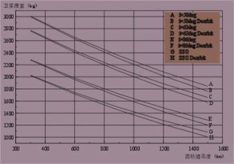
Figure 12. Launch capability of Long March 2C.

The other physical limit on launch capability is dimensions of the launch vehicle’s fairing. Fairing is where the payload of the launch vehicle is stored. The satellite to be launched must fit in the fairing or otherwise it cannot be launched even if its mass is lower than the vehicle’s lifting capability. Figure 13 shows a typical fairing diagram. From the data provided by the diagram, the volume of the fairing can be easily estimated. By comparing the volume of the satellite with the internal volume of the fairing, we will know whether the fairing can accommodate the satellite.

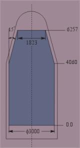
Figure 13. Fairing dimensions of Long March 2C.

LVM checks the satellite design against the three limits mentioned above: inclination, altitude, and fairing dimension. If the satellite design is within the range of these limits, then we interpolate the type of diagrams in Figure 12 to find the payload mass the launch vehicle can lift to the designed orbital altitude. If the payload mass is larger than satellite mass, and the fairing volume is larger than satellite volume, then the launch vehicle is recognized as a capable vehicle and added to an array recording capable launch vehicles. To find how many satellites can be sent up per vehicle (SPV), we use the following simple expression, in which M_PL is payload mass, V_fairing is fairing volume, M_sat is satellite mass including insertion fuel, and V_sat is satellite volume including insertion fuel,

(52)

so that the lower of the mass limit and volume limit is taken. The number of launches to send up the entire constellation is found as

(53)

The information sources for launch capabilities also give the cost per launch for each launch vehicle. Then the total launch cost C_launch is simply

(54)

After checking the capabilities of all six launch vehicles, the array recording the capable launch vehicles and their cost information is scanned. The capable vehicle with lowest cost is chosen to be the selected launch vehicle for the design, and its information and technical data are returned to SF.

Since launch vehicles such as Ariane 5 can lift 6 tons of payload to the geostationary transfer orbit (STO), it is hard to imagine any design is unable to find a launch vehicle capable of lifting it to the much lower LEO orbits. In the unlikely event that the satellite cannot find a capable launch vehicle, SF will set its capability in term of simultaneous users supported by a satellite to zero. Otherwise, the satellite capability needs to be calculated in the capacity modules as introduced in the following section.

Capacity Modules (CM)

The capacity modules calculate the number of simultaneous users a satellite can support. As described in Unit 1, there are two major types of modulation schemes: MF-TDMA and MF-CDMA. Each scheme requires a different approach in capacity calculation. Therefore, CM is divided into five subroutines. The first three subroutines together calculate the capacity of MF-TDMA scheme, and the rest two subroutines calculate the capacity of MF-CDMA scheme. Before introducing the computer codes, we will look at the mathematical equations for the capacity calculation. In the paragraphs below, I will just give the final equations that are used in the code. A paper has been written to describe the physics behind these equations and to give a more thorough derivation.[15]

For MF-TDMA, we first need to find the total data rate for FDMA carriers per cell. There are two possible limits on the data rate – power limit and bandwidth limit. The FDMA data rate per FDMA carrier due to power limit can be calculated using link budgeting, where R_FDMA stands for data rate per FDMA carrier, Power_cell for transmitter power per cell, N_FDMA for number of FDMA carriers per cell, G_t for transmitter gain, G_r for receiver gain, k for Boltzmann’s constant, T_s for system temperature, E_b/N₀ for bit energy to noise ratio, L_tot for total loss along the transmission path, and margin for link margin

(55)

Moving N_FDMA to the left-hand side of the equation gives the total data rate of all the FDMA carriers per cell defined by power limit

(56)

To find data rate per cell due to bandwidth limit, we first write the data rate per FDMA channel defined by bandwidth limit. Let BW_cell denotes bandwidth per cell (= satellite bandwidth / cluster size), M denotes signal modulation level, β for Nyquist filter rolloff factor, normally ranging from 0.2 to 0.5, B_T for frequency channel bandwidth, and B_g for guard bandwidth, then

(57)

Moving N_FDMA to the left-hand side of the equation gives the total data rate of all the FDMA carriers per cell defined by bandwidth limit

(58)

In this equation, we already know BW_cell; M is 4 if QPSK is used, and β is set to 0.26 as a constant. In Iridium, the frequency domain is divided so that

(59)

We assume this division applies to all MF-TDMA systems and use the value of 0.9712 in Equation (58).

To find the number of TDMA channels, we refer to the geometry of time distribution as shown in Figure 4 of Unit 1. In the geometry, let FL denote frame length, FIL denote framing time slot length, TGL denote total guard slot length, and R_user denote individual user datarate. It is not difficult to perceive the following relation

(60)

Per theory of MF-TDMA modulation scheme, the total number of MF-TDMA channels is the product of N_FDMA and N_TDMA. Then we will get

	(61)

In this equation, N_FDMAR_FDMA is the lower of the results from Equation (56) and (58). To find the fractional term in the equation, we use the design of Iridium and assume it is typical of MF-TDMA systems. In Iridium, the time domain is divided so that

(62)

Therefore, the capacity of a MF-TDMA system can be found. For Iridium, equation (61) gives a capacity of 905 simultaneous users per satellite.

For MF-CDMA system, omitting the detailed derivations, we arrive at an equation for the number of simultaneous users per cell N_c, where T denotes number of CDMA carriers in the satellite bandwidth, B_sat denotes satellite bandwidth, B_g denotes guard band between CDMA carriers, R_user denotes individual user data rate, α of value 0.5 represents the expected value of voice channel activity state, f denotes neighboring user interference factor, E_b/N₀ represents the ratio of bit energy to noise caused along the link, and E_b/I_tot represents the ratio of bit energy to noise including both N₀ and interference noise.

(63)

and an equation for E_b/N₀ for each individual link is

(64)

or, if move N_c to the left-hand side,

(65)

Substituting (64) into (63) and solve for N_c, we find the following expression

(66)

As I mentioned before introducing the equations, five subroutines are written to convert the above mathematical expressions into the simulation. The first three subroutines are for MF-TDMA, among which, the first subroutine linkRate.m returns the value of R_FDMAN_FDMA in (56). The second subroutine BWLimit.m returns the value of R_FDMAN_FDMA in (58). The lower of these two values defines the bound and is input into the third subroutine MF_TDMA.m, which uses (61) to find the total number of MF-TDMA channels supported by a satellite.

The next two subroutines find the capacity of a MF-CDMA system. The first of them linkEbNo.m gives (E_b/N₀)N_c in (65). Substituting this result to the last subroutine MF_CDMA.m, N_c in (66) is calculated. The satellite capacity is the product of N_c and the number of cells N_cell calculated in (24).

(67)

One more thing worth mentioning despite the omission of the derivation of the equations is convolutional coding. In convolutional coding, redundancy cleverly coded into transmitted information reduces transmit power required for a specific bit error probability. This reduction process has two important parameters, code rate r and constraint length K. Code rate r is defined by the ratio between the original information bits k and the redundantly coded content bits n,

(68)

The bit energy to mean total noise power spectral density ratio E_b/I_tot corresponding to several bit error probabilities, p_b, are listed in Table 8 for soft-decision Viterbit decoding.[16]

pb	Eb/Itot uncoded	Rc = 1/3		Rc = ½			Rc = 3/3		Rc = 3/4
		K = 7	K = 8	K = 5	K = 6	K = 7	K = 6	K = 8	K = 6	K = 9
10^-3	6.8	4.2	4.4	3.3	3.5	3.8	2.9	3.1	2.6	2.6
10^-5	9.6	5.7	5.9	4.3	4.6	5.1	4.2	4.6	3.6	4.2
10^-7	11.3	6.2	6.5	4.9	5.3	5.8	4.7	5.2	3.9	4.8

Table 8. Coding gain E_b/N₀ (dB-b^-1) for soft-decision Viterbi decoding, QPSK

From table like this, the values of E_b/N₀ in (56) and of E_b/I_tot in (66) can be read and used in the simulation.

The satellite capacity of either the MF-TDMA system or MF-CDMA system is returned to SF. Then in SF, the system capacity in term of the number of simultaneous users supported by the entire constellation is calculated. The calculation is slightly different for polar constellation and Walker constellation. Because satellites in the polar constellation all need to fly above the poles, at the poles there is a severe overlapping of satellites’ footprints. This overlapping causes a reduction in the overall system capacity of polar constellation, which can be represented by the polar overlapping factor (POL)of 0.68 for polar constellation. For Walker constellation, POL is 1 because Walker constellation covers only below certain latitude and never passes the poles. Therefore the system capacity equation is

(69)

Total Cost Module (TCM)

The cost module methodically computes the present value of the life-cycle cost of the system. The method is modified on the basis of cost estimating relationships (CERs) in SMAD. A step-by-step introduction to the method will be given after we introduce the inputs and output of the module. The inputs include the number of satellites in the constellation, number of orbital planes, orbital altitude, antenna weight, communication electronics weight, spacecraft bus dry weight, satellite mass (wet weight), beginning-of-life power, flight software thousand lines of code, ground software thousand lines of code, designed life of space segment, initial deployment time, number of gateways, number of operations and support personnel, AKM type, AKM dry weight, AKM impulse, discount rate, minimum launch cost, and ISL datarate. The output of the module is the total present value of the life-cycle cost (LCC) of the designed system. All cost terms in this module are in unit of thousand of U.S. dollars in fiscal year 2002.

In this module, it takes totally 16 steps to account for the LCC of the system. The first step sets space mission characteristics. Most of these characteristics are design variables, constants, or system parameters obtained in previous modules. There are two exceptions: payload type and number of spare spacecraft. Apparently, the payload type is communication. A spare satellite is typically launched into each orbital plane at altitude lower than that of the regular orbit so that it is ready to replace a failed satellite in that orbital plane. Therefore the number of spare spacecraft is set to the number of orbital planes.

The second step accounts for the hardware cost of the research, development, test and evaluation (RDT&E) phase. As the name suggests, this phase occurs very early in the system life-cycle. It is a breakdown of the costs of antenna, communication electronics, spacecraft bus, and apogee kick motor. Each cost is in relation with the weight of that particular component except that the AKM cost is linear with the AKM impulse.

If antenna weight is M_ant, then the antenna cost is found to be

(70)

The communication electronics cost is

(71)

where CEW is weight of communication electronics. The cost of spacecraft bus is based on SCBDW, the dry weight of spacecraft bus

(72)

The AKM weight depends on AKM impulse and also on the AKM type. If the AKM is spin-stabilized, then the cost is

(73)

If the AKM is 3-axis stabilized, which is more popular for current LEO communication satellite design, then the cost is

(74)

The total hardware cost of the RDT&E phase is the sum of the above component costs. Because the relations above are developed using 1992 USD value, I have converted them to 2002 USD value by the inflation rate of 1.369. Therefore the hardware cost is

(75)

The third step is to find to find theoretical first unit (TFU) hardware cost. This step is same as the previous step except the component costs are calculated different as what follow

(76)

(77)

(78)

For spin-stabilized AKM,

(79)

For 3-axis stabilized AKM,

(80)

The rest of step 3 is the same as step 2. The TFU hardware cost is

(81)

Step 4 is to find the hardware cost of every spacecraft produced. This step includes the learning curve phenomenon that accounts for production cost reduction as the production quantity increases. The reduction in cost is due to economies of scale, set up time, and human learning. The total production cost of N units is modeled as

(82)

The learning curve slope S represents the percentage reduction in cumulative average cost when the number of production units is doubled. SMAD recommends the following values for learning curve slope.

Number of units	Learning curve slope
≤10	95%
10< and ≤50	90%
50<	85%

Table 9. Learning curve slope values

The cost of the first unit is C₁ given by equation (82) with N = 1; the cost of the second unit is C₂ – C₁ where C₂ is given by equation (82) with N = 2; the cost of the third unit is C₃ – C₂ – C₁, so on and so forth. The hardware costs of all units are assigned to elements of an array called UHC.

Step 5 finds aerospace ground equipment cost for RDT&E. The cost is expressed in a simple linear relation

(83)

Step 6 finds total program level cost for RDT&E and all units including TFU. First, program level cost for RDT&E is

(84)

Program level cost for all units is

(85)

Total program level cost is

(86)

Step 7 is to find launch operations and orbital support cost. For launch without the use of AKM, the cost per satellite is

(87)

For launch with AKM, the cost per satellite is

(88)

The total cost of all satellite units is

(89)

Step 8 finds flight software cost by scaling the thousand lines of code.

(90)

Step 9 account for the minimum launch cost found in the launch vehicle module.

(91)

Step 10 finds ground software cost assuming the language used is Unix-C.

(92)

Step 11 is to find total ground segment development cost, which is consisted of costs of all the gateways and two command centers. SMAD suggests that the cost of developing a gateway (or ground station) has a breakdown as listed in Table 10.

Ground Station Element		Development Cost as Percent of Software Cost (%)
Facilities (FAC)		18
Equipment (EQ)		81
Software (SW)		100
Logistics		15
System level
	Management	18
	Systems engineering	30
	Product assurance	15
	Integration and test	24

Table 10. Ground segment development cost distribution

So the ground station development cost is simply

(93)

In addition to gateways, the system also needs command centers to control network and satellite operations. Two command centers are assumed for the system. The cost of each command center is the average of seven actual systems’ command center costs drawn from their FCC filings. These seven systems are @contact, ARIES, GEMnet, Globalstar, Orbcomm, Starnet, and VITA. The average cost is 11.856 million USD. Therefore the total ground segment development cost is the sum of the costs of all the gateways and two command centers.

(94)

Step 12 is to find initial development cost (IDC), which is the cost up to the onset of the service of the system. To get IDC, we need to sum up all the costs we have calculated previously.

(95)

In order to find the present value of the cost, a cost distribution over development time needs to be modeled first. To be clear, the life-cycle of the system is consisted of two stages. The first stage is the initial development time (IDT) that starts with the RDT&E stage of the system, and extends till the deployment of the entire system. The second stage is the space segment life, which starts with the completion of system deployment and onset of service, and lasts until the end life of the satellites. In step 13 we look at the cost distribution in IDT. SMAD suggests to find the cost spreading by a function of the form

(96)

where F(S) is the fraction of cost consumed in time S, S is the fraction of the total time elapsed, and A and B are empirical coefficients. Coefficients A and B depend on percentage of expenditure at schedule midpoint. For project involving more than two satellites, 50% expenditure at schedule midpoint is suggested, and the corresponding A and B are 0 and 1.00. Using these values, it is easy to find the cost per year for each year during the IDT. These values are stored in array C_year. As mentioned above, we assume the IDT to be a constant at 5 years.

Step 14 gives operation and support cost per year during space segment life time. The yearly maintenance cost per gateway is

(97)

For personnel cost, contractor labor is estimated to cost $140K/staff year. Also 300 staff members are assumed to keep the business running, besides the personnel at the gateways. Summing the maintenance and personnel costs, the total operation and support cost per year is

(98)

In step 15, C_{OS per year} is distributed over space segment life time. Because the maintenance and personnel costs are assumed constant throughout the years, we simply assign the value of C_{OS per year} to each year in the space segment life time. After appending the space segment life time yearly cost to it, C_year covers the entire life-cycle of the system.

(99)

In step 16, an additional fee is accounted as 10% of the total cost. So the final total cost C_tot is

(100)

The value of the total cost is returned to SM.m as the life-cycle cost.

Market Module (MM)

MM estimates the number of subscribers to the service provided by the satellite system per year, the total air time of the system, and the total amount of data transmitted throughout the system’s lifetime. These are the outputs of the module. The inputs of the module are number of users supported per satellite, number of satellites in the system, footprint area, initial development time, space life of the system, and data rate per user.

The first part of the module is to model the total global potential user (GPU_tot) throughout the space lifetime of the system. The initial development of the system is assumed to start in 2004. The global potential user (GPU) in the first year of the service (in millions of subscribers) is

(101)

where A is the number of subscribers in 2003, B is the yearly increment of subscribers, IDT is the initial development time, and IDT + 1 is the first year of service. The number of total potential users in the last year of the service is

(102)

The total number of global potential users throughout the life time of the system is

(103)

For this study, we model the market for both low-bandwidth satellite system and high-bandwidth system. If the user data rate is lower than 50 kbps, then the system is considered as a low-bandwidth system; otherwise it is a high-bandwidth system. The market data for low-bandwidth system is based on the FCC filing of Globalstar, which is also a low-bandwidth system. Market projection for high bandwidth satellite service is provided by Pioneer Consulting. The values of A and B for the two types of systems are listed in Table 11.

	A (Million potential subscribers in 2003)	B (Yearly increment of million potential subscribers)
Low-bandwidth system	49.60	2.97
High-bandwidth system	4.92	0.52

Table 11. Market projections for low-bandwidth and high-bandwidth systems

Earth land area is 148.326 million square kilometers. I assume the potential users distribute evenly over the land area indiscriminant of developed or developing regions. The reasoning for an even distribution is that in developed regions, although more people can afford the service, a small percentage of this people have an incentive to subscribe to satellite service because the terrestrial system has been in place; in developing or under-developed regions, although few people can afford the service, a large percentage of the people who can afford it have an incentive to purchase the service because terrestrial system has not been in place to provide competitive service. So the number of potential subscribers per square kilometer is

(104)

The satellite capacity is evenly distributed over the entire earth surface. Earth surface area is 4πR_e². So the number of subscribers per square kilometer supportable by the satellites is

(105)

The number of actual subscribers per square kilometer is the smaller of the two

(106)

The total number of subscribers is

(107)

The average number of subscribers per year is

(108)

If each subscriber is assumed to use the service one hour everyday, 365 days a year, then the total air time throughout the system lifetime (in minutes) is

(109)

Total data flow throughout the system lifetime (in MB) is

(110)

This module returns the values of average number of subscribers per year, total air time, and total data flow to SF.

Output assignment and Postprocessing

The market module is the last module in the simulation. After the execution of the market module, we are back in the nested for-loops. The last step in the for-loops is to assign the values of the objectives to the objective vector J, the benchmarking parameters to B, and requirements to r. This concludes the nested for-loop.

The post-processing is carried out at the end of SF. It involves finding the Pareto front and the utopia point of the design space. These two characters of the design space exploration will be introduced in the design space exploration and optimization section below. Before we explore the design space, benchmarking should be performed to prove the fidelity of the simulation.

References

---

[1] Jilla C, Miller D.

[2] Ross A., Hastings D.,

[3] For the full-factorial case where combinations of different design variable values are run, we assume the frequency bands are same as those for Iridium.

[4] Jilla, C.

[5] Recall that the communications performance (i.e. the quality of service) is held constant for each channel of these systems, by virtue of the requirements vector, r.

[6] O.L. de Weck and K. Wilcox. ESD.77 Multidisciplinary System Design Optimization (MSDO), Massachusetts Institute of Technology. Lecture 13 Multi-objective Optimization (I), 8 April 2002.

[7] De Weck, Isoperformance

[8] The theoretical part of this section is based on O.L. de Weck and K. Wilcox. ESD.77 Multidisciplinary System Design Optimization (MSDO), Massachusetts Institute of Technology. Lecture 11 Solution Sensitivity Analysis, 1 April 2002.

[9] The derivation of equations for the polar constellation is based on E. Lutz, M. Werner, and A. Jahn. Satellite Systems for Personal and Broadband Communications. Springer-Verlag, Berlin, Germany, 2000.

[10] Lang, T.J., and Adams W.S., "A Comparison of Satellite Constellations for Continuous Global Coverage", paper 1.4, IAF International Workshop on Mission Design and Implementation of Satellite Constellations, Toulouse, France, Nov 17-19, 1997.

[11] The data are listed in Table 13-16 in W.J. Larson and J.R. Wertz. Space Mission Analysis and Design. Microcosm, Inc., Torrance, CA, 1992.

[12] S.J. Isakowitz, J.P. Hopkins Jr., and J.B. Hopkins. Reference Guide to Space Launch Systems. AIAA, Reston, VA, 1999.

[13] China Academy of Launch Vehicle Technology (CALT) official website English version. http://www.calt.com.cn/new/english/ [4 August 2003].

[14] Arianespace official website. http://www.arianespace.com/site/index2.html [4 August 2003].

[15] D.D. Chang and O.L. de Weck. Basic Capacity calculation methods and benchmarking for MF-TDMA and MF-CDMA communication satellites. 21^st AIAA International Communications Satellite System Conference (ICSSC) and Exhibit, 2003.

[16] J.E. Kadish and W.R. East. Satellite Communications Fundamentals. Artech House, Boston, 2000.