Instructor
Anastasia Yendiki, Ph.D.
Lab description
The purpose of this lab is to familiarize you with
spatial normalization and perform joint statistical analysis
of data that has been collected from a single subject
but multiple runs of the same functional paradigm.
Lab software
We will use NeuroLens
for all fMRI statistical analysis labs.
Lab data
We will use data from the self-reference functional paradigm
that was presented in Lab 1. For this lab we will use all data
from Subject 7, available under the course directory:
/afs/athena.mit.edu/course/other/hst.583/Data2006/selfRefOld/Subject7Sessions7-8-9-13/
Here's a reminder of the paradigm structure.
Words are presented in a blocked design.
Each run consists of 4 blocks,
2 with the self-reference condition and
2 with the semantic condition.
The conditions alternate in the ABBA format.
In particular, for Subject 7 the order is:
Run 1:  A=semantic, B=selfref
Run 2:  A=selfref,  B=semantic
Run 3:  A=semantic, B=selfref
Run 4:  A=semantic, B=selfref
Words are presented for 3 sec each, grouped in blocks of ten. Prior to each block the subject views a 2 sec cue describing their task for the upcoming block. Each block is followed by 10 sec of a rest condition. This is the breakdown of a single run:
10 sec   Rest
2 sec    Cue
30 sec   Block A (10 words, each lasts 3 sec)
10 sec   Rest
2 sec    Cue
30 sec   Block B (10 words, each lasts 3 sec)
10 sec   Rest
2 sec    Cue
30 sec   Block B (10 words, each lasts 3 sec)
10 sec   Rest
2 sec    Cue
30 sec   Block A (10 words, each lasts 3 sec)
16 sec   Rest
----------------------------------------
TR = 2 sec
Total run duration = 184 sec (i.e., 92 scans) per run
Lab report
The lab report must include your answers to the questions found
throughout the instructions below.
Due date: 12/04/2006
-
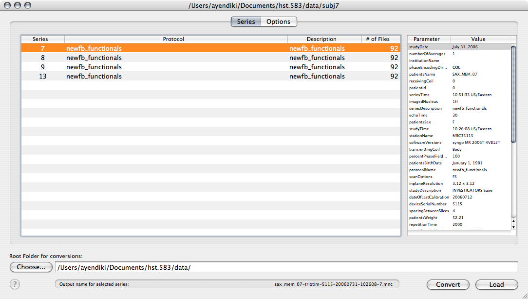
As usual, open the Subject 7 data by dragging its entire folder onto the NeuroLens icon (or by starting NeuroLens and choosing Open... from the File menu):
-
After the preliminary exploration of the data from run 1 in previous labs, we will now proceed with the analysis of all four runs of the self-reference paradigm from Subject 7.
In the first lab you created a text file that contained the timing of the self-reference and semantic conditions as they appeared in runs 1, 3 and 4. Now create a similar file for the timing of run 2 and save it with a name like selfref,run2.txt.
-
We will pre-process and fit a linear model to the functional EPI images from each run separately. We will save the outputs of the linear model fit that will be needed to perform a second-level analysis on all four runs.
For each of this subject's four runs, open the corresponding EPI image set and perform the following steps:
-
Motion-correct the images.
-
Apply spatial smoothing to the motion-corrected images, using a Gaussian smoothing kernel with a FWHM of 6mm.
-
Normalize the intensity of the smoothed images to a mean value of 10000: From the Action toolbar item, choose Intensity Normalization, set the Normalization target value to 10000 and click on the OK button. This step is needed because we will average results from different runs (and, in the next lab, different subjects).
-
Fit a linear model to the normalized images. Use the appropriate design matrix for the run that the image set came from. Use the default HRF shape and the same maximum order of the polynomial drift terms as in the previous lab (1). Set up a single contrast, that of the self-reference condition vs. the semantic condition. Configure the linear model to output the measures that are required for a second-level analysis. (In the Output tab, check Effect size and Standard error for effect.) You will not need individual T-maps or other outputs from each run.
-
Save the resulting volumes of effect size and effect standard error to disk, choosing names that indicate the subject and run that they correspond to.
-
Leave the window showing the normalized EPI volume series open because you will need it for the next step.
-
-
We will now register the EPI volumes from each run to a standard EPI brain average that is available in NeuroLens. This involves running a volume registration algorithm that will calculate the shift, rotation, shearing, and scaling that must be applied to the EPI volumes from each of our subject's runs so that they are mapped to the space defined by the standard EPI brain. We will then save the calculated shift, rotation, shearing, and scaling parameters so that we can apply them to the outputs of the linear model fitting that we performed in the previous step.
Perform the following steps on the EPI volume series from each of the four runs:
-
Go to the window showing the pre-processed EPI volume series (the one that was the input to the linear model fitting in the previous step). From the Action toolbar item, choose Volume Registration. The Volume Registration window will pop up, showing the steps that the registration algorithm will follow to find a mapping from the space of the current EPI volume series to the target space:
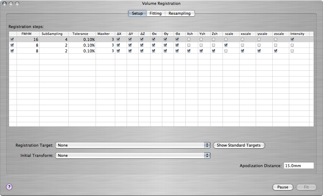
For each of the three steps, you can control
- How much the source and target, i.e., the subject's brain and the standard brain, are smoothed at that step (FWHM)
- How much coarser the resolution of the two brains is made at that step (SubSampling)
- Which of the registration parameters are allowed to vary at that step: Shift along each dimension (ΔX, ΔY, ΔZ), rotation angle around each axis (Θx, Θy, Θz), shearing in each dimension (Xsh, Ysh, Zsh), overall scaling (scale), scaling in each dimension (xscale, yscale, zscale), and image intensity (Intensity).
For now we will use the default settings.
-
To specify that the space of the NeuroLens standard EPI brain is the target space for this registration, click on the Show Standard Targets button. In the popup window that shows up, select the file named 3T-EPI-Target.mnc and click on the Open button. A new window will open that displays the standard EPI brain. To examine whether the standard brain and the brain of Subject 7 are well-aligned, command-click on various anatomical landmarks in the standard brain and check if the cursor has moved to the corresponding landmark in the brain of Subject 7:
-
Go back to the Volume Registration window. Click on the Fitting tab and then click on the Fit button to start the registration. When the Progress box shows Current Registration Phase: Finished, the registration is done. The Fitting tab shows overlays of the source and target volumes. When the registration is done, move the slider next to the overlays up and down to check how well the registered volumes match each other.
-
So far we have only computed the registration parameters, but we have not applied them to our subject's brain to map it ("resample" it) onto the space of the standard brain. We will do this now, because it will help us check the quality of the registration.
Click on the Resampling tab. From the menu on the left, labeled Sample data of, choose the subject's EPI volume (the one from which you started this registration). From the menu on the right, labeled at voxel locations of, choose the standard EPI brain volume (3T-EPI-Target.mnc).
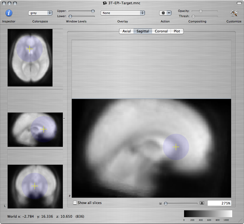
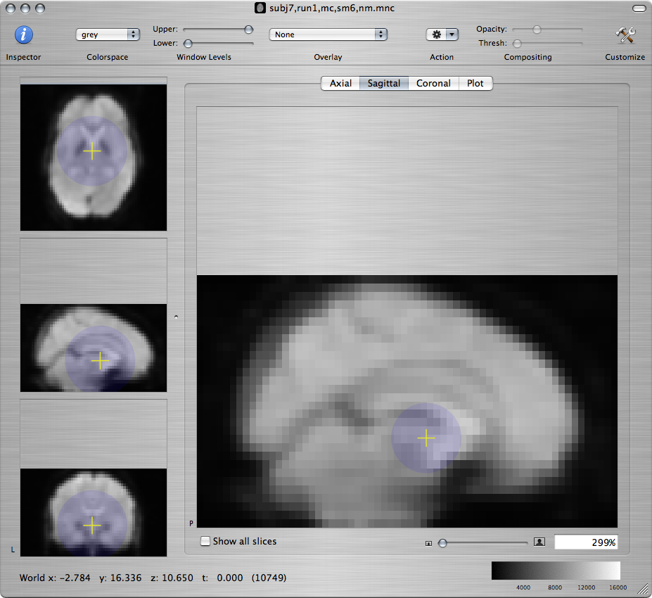
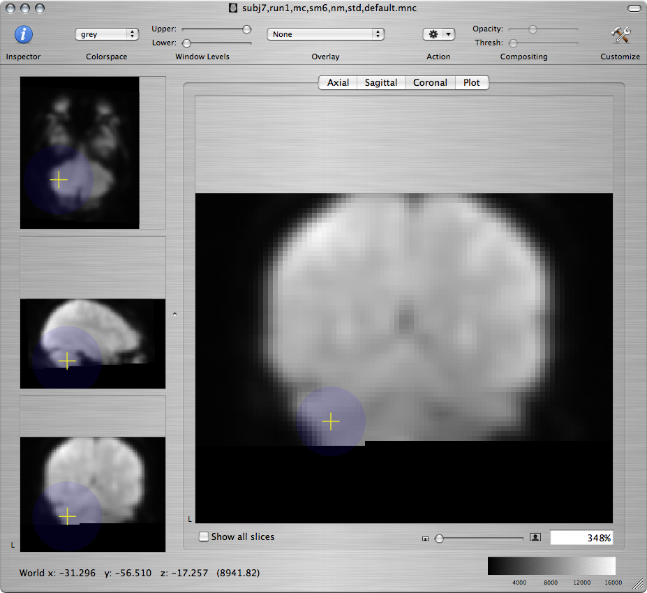
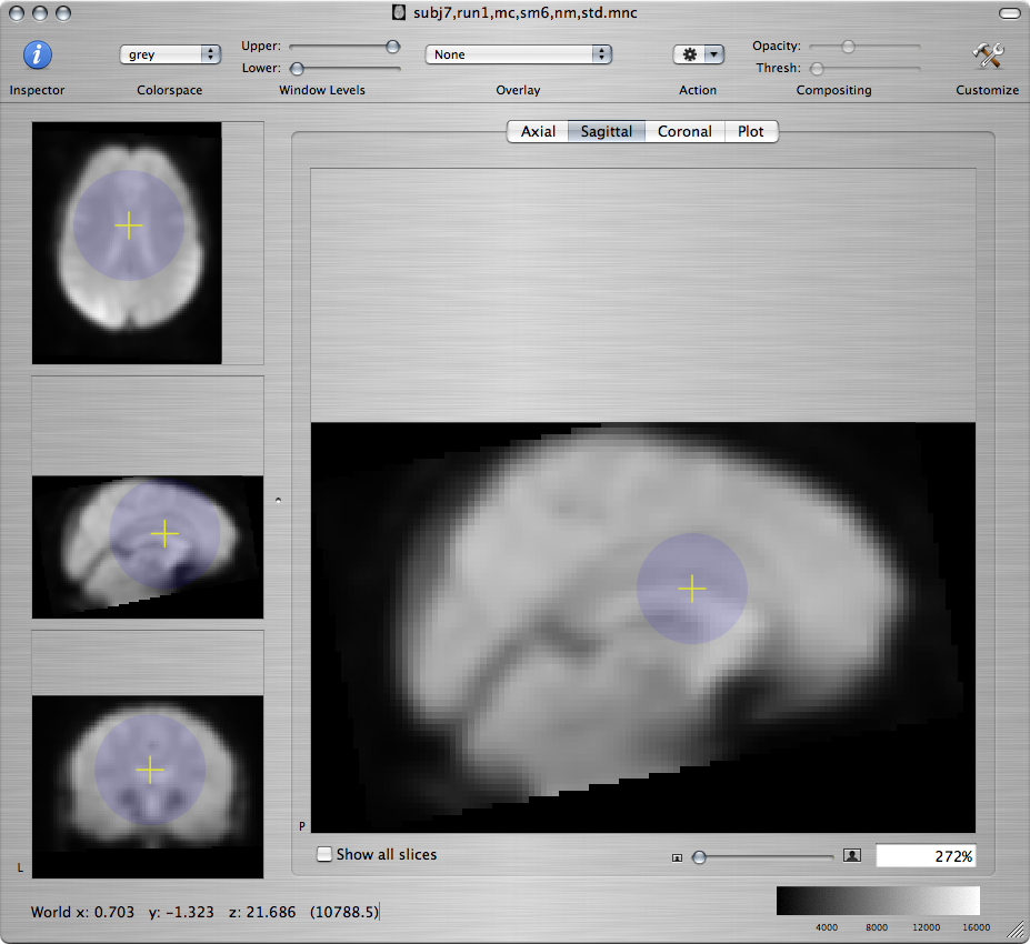
Click on the Resample button. A new window will appear, showing the subject's EPI volume mapped onto the space of the standard EPI brain. To check the quality of the registration, you can now command-click on various landmarks in the window of the standard brain and check if the cursor moves to the corresponding landmark in the window of the subject's resampled brain. Good landmarks are anatomical features that appear clearly darker or lighter than their surroundings.
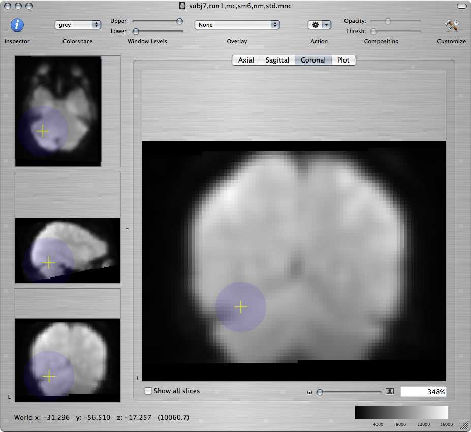
For example, on a coronal view command-click near the edges of the cerebellum:
Standard brain Resampled subject - bad Resampled subject - better 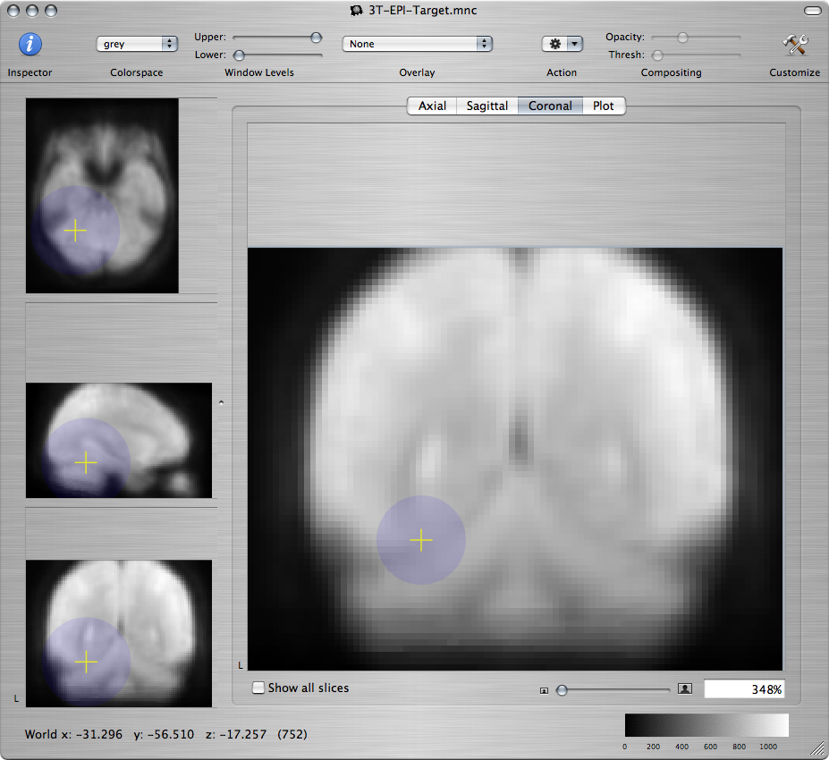
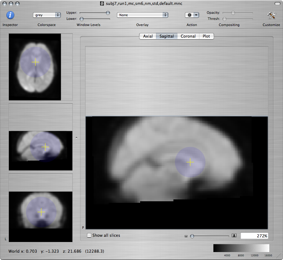
Or, on a sagittal view command-click along the medial wall:
Standard brain Resampled subject - bad Resampled subject - better 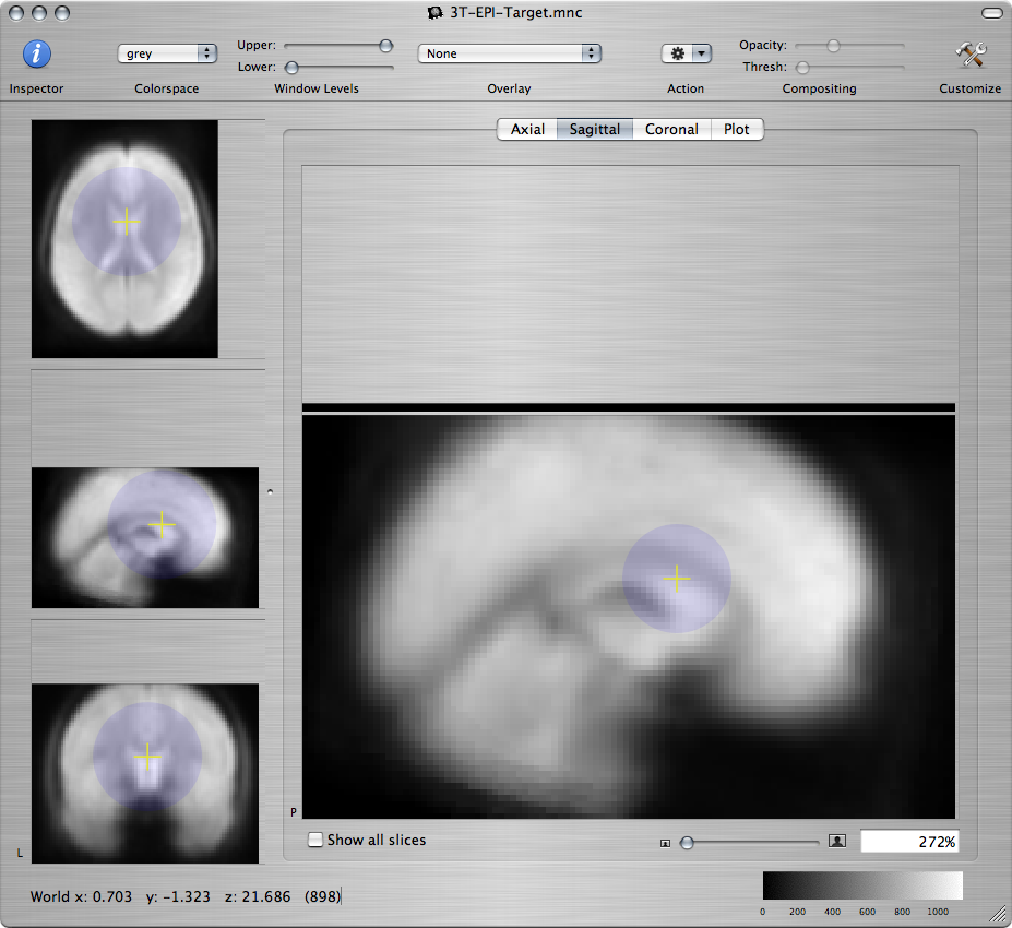
-
If the registration is not good, try changing the parameters in the Setup tab of the Volume Registration window and repeat the registration.
Hints: If some of the registration parameters (shifting, scaling, etc.) look like they are off, you can allow them to vary during more than one step of the registration. Or, you can reduce the amount of smoothing and/or subsampling during one or more of steps to refine the registration. These changes will typically make the registration slower, but they may help improve the final result. When you see that a registration is progressing in a bad direction, you can click on the Pause button and start over without waiting for it to finish.
Q: Once you have a registration that you are satisfied with, report the setup of the 3 registration steps from the Setup tab that you used to obtain this registration. Provide screenshots that illustrate the agreement between the source and target volumes. There is no perfect answer!
Once you have improved that registration as much as you can, try registering the unsmoothed EPI images (after motion correction, but before spatial smoothing) to the standard EPI brain.
Q: How does the registration of the unsmoothed images compare to that of the smoothed images? Why?
Note: Once you have registered the images from the first run, you can decide which registration approach gives you the best results (i.e., decide if you should register the smoothed or unsmoothed image set, and decide what setup to use for the three registration steps). Then you can follow the same approach when registering the remaining three runs. However, you will need to register each of the runs separately, since the subject may have moved between runs.
-
After you have settled on a registration that you are satisfied with, it is a good idea to save the tranformation parameters in case you need to reuse them. In the Fitting tab of the Volume Registration window, click on the Open transform button to display the estimated transformation parameters. While the parameter window is current, go to File > Save as... and save the transformation to a file. Choose a file name that indicates the subject and run that you are processing.
-
Next you will resample the effect size and effect standard deviation that you obtained by fitting a linear model to this run's EPI series.
Make sure that the effect size and effect standard deviation volumes from this run are open. Go to the Resampling tab of the Volume Registration window and resample each of these two volumes to the standard brain, using the good transformation that you have just saved. Save the resampled effect size and the resampled effect standard deviation.
-
-
We are now ready to perform a second-level analysis (group analysis) that will combine the data from this subject's runs. We will gradually decrease the number of runs that we include in the analysis and record the change in statistical power in different ROIs.
Make sure that the resampled effect size volume and the resampled effect standard deviation volume from each of the four runs is open. Go to the window displaying one of the resampled effect size volumes. From the Action toolbar item, choose Group Analysis. The Group Analysis window will open, showing a list of the effect size volumes from the four runs:
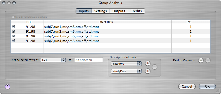
The last column must have a value of 1 for each of the runs that will go into the group analysis, so that the analysis tests for significant non-zero values in the average of the runs.
In the Settings tab, choose the Analysis type to be Pure fixed effects.
In the Outputs tab, check the -log(p) box.
Click on the OK button to perform the group analysis and save the resulting -log(p) map.
-
Repeat the group analysis, but this time in the Inputs tab uncheck the checkbox next to the effect size file from the 4th run, so that you include only the first 3 runs in the analysis. Save the resulting -log(p) map.
-
Repeat the group analysis, now including only the first 2 runs. Save the resulting -log(p) map.
-
The group analysis cannot be performed with only one run. Fit a simple linear model to the pre-processed images from the first run to obtain a -log(p) map of the self-reference-vs.-semantic contrast.
Resample this map to the space of the standard EPI brain, using the transformation file that you saved when you registered the EPI series from the first run to the standard EPI brain. (You will need to open that transformation file so that you can select it in the Resampling tab of the Volume Registration module.) Save the resampled -log(p) map. This map can now be compared directly to the ones you obtained from the group analyses, as they are all in the space of the standard brain.
-
Make sure that the four -log(p) maps that you obtained by averaging 4, 3, 2, and 1 run(s) respectively in steps 5-8 are open.
You will now measure the maximum value of these maps in 3 different ROIs along the medial wall. Open the ROIs:
- /afs/athena.mit.edu/course/other/hst.583/Data2006/selfRefOld/subj7,std,roi1,lab7iii.mnc
- /afs/athena.mit.edu/course/other/hst.583/Data2006/selfRefOld/subj7,std,roi2,lab7iii.mnc
- /afs/athena.mit.edu/course/other/hst.583/Data2006/selfRefOld/subj7,std,roi3,lab7iii.mnc
Using the ROI Statistics module from the Action toolbar item as you did in the previous lab, find the maximum value in each of these ROIs in each of the four -log(p) maps.
Number of runs in analysis Max -log(p) ROI1 Max -log(p) ROI2 Max -log(p) ROI3 1 2 3 4 Q: Show plots of the maximum -log(p) value vs. the number of runs included in the analysis, for each of the three ROIs. What trend do you observe? How do you explain this finding?
-
Q: What regions of the subject's neuroanatomy do these ROIs correspond to? You can overlay the ROIs on the standard brain and consult the slides from Lab 1 to help you answer this question.
| < Previous lab | Next lab > |