A NEURON Programming Tutorial - part C
Introduction
At the beginning of part A, we
defined our final product to be a model of a small network of
rat subthalamic nucleus projection neurons with each neuron
having a particular dendritic tree morphology.
In this part, we will explore how to introduce 3D spatial
information into the model (i.e. where to place in 3D space
dendrites and neurons), how to define multiple neurons using
templates, and how to connect neurons up using
NetCon.
Templates
In part B, we created the first
neuron that we need in our subthalamic network system. In this
example we will create only 4 neurons, but we will create them
in a way that increasing the number of neurons in our network
is easy later on.
We need to copy the neuron we have already created to create
additional neurons. NEURON provides us with
a simple way to create multiple copies of the same neuron:
templates.
A template is an object definition--it defines a
prototype of an object from which we can create multiple
copies. After defining the template, we must declare the object
variable that we will use to reference the objects, just as we
have in the past with the IClamp. Then, we can create
a new instance of the object from the template that is an exact
copy of the template. After we create the object from the
template, we can either use it as it is or we can modify it to
fit our needs. The structure of a template is as follows:
begintemplate name
code
endtemplate name
where name is the name of the template we
want to create, and code is any program
commands that we want the template to include.
Here is a long definition of a template that illustrates
several aspects of templates.
begintemplate SThcell
public soma, dend

create soma, dend[1]

proc init() {

    ndend = 2

    create soma, dend[ndend]

    soma {
      nseg = 1
      diam = 18.8
      L = 18.8
      Ra = 123.0
      insert hh
      gnabar_hh=0.25
      gl_hh = .0001666
      el_hh = -60.0
    }

    dend[0] {
      nseg = 5
      diam = 3.18
      L = 701.9
      Ra = 123
      insert pas
      g_pas = .0001666
      e_pas = -60.0
    }

    dend[1] {
      nseg = 5
      diam = 2.0
      L = 549.1
      Ra = 123
      insert pas
      g_pas = .0001666
      e_pas = -60.0
    }

    // Connect things together
    connect dend[0](0), soma(0)
    connect dend[1](0), soma(1)
}
endtemplate SThcell
Creating new neurons from this template is straightforward.
If we define an array of object variables:
nSThcells = 4
objectvar SThcells[nSThcells]
we can then create all four of our cells using the new command in a for
loop:
for i = 0, nSThcells-1 {
    SThcells[i] = new SThcell()
}
Each cell is a complete subthalamic neuron as we had
described at the end of part B.
We will describe two main features of this template
example:
-
The public statement is used
to tell NEURON what parts of the
template can be accessed outside of the template
definition. Normally, if there are no public
names, then the code inside the template is completely
private and nothing, aside from the name of the template
itself, is accessible from the rest of the program code.
For example, if we create a neuron template and we want to
be able to put a current clamp in the soma of the neuron we
create, we would need to give access to the soma
section via the public command.
After declaring the neurons with the objectvar command and creating the objects with
the new command, we can access a
neuron soma using dot notation (e.g.,
SThcells[2].soma.L is the length of the soma in
the 3rd neuron we created). In this template example both
soma and dendrites are public allowing us to access them
both through the dot notation. We can now insert
current clamps into all of our neurons as follows:
objectvar stim[nSThcells]

for i = 0, nSThcells-1 SThcells[i].soma {
    stim[i] = new IClamp(0.5)
    stim[i].del = 100
    stim[i].dur = 100
    stim[i].amp = 0.1
}
-
The init() procedure. Most
templates will have a special procedure called
init() which is automatically called when a new
object is created from the template. This is very useful to
initialise the newly created object. In our init()
procedure, above, we have created and defined all the
sections in our neuron and appropriately connected them
together. Thus when a neuron object is created from the
template with the new command an
entire subthalamic neuron is built.
Arguments to
init()
Arguments can be passed to init() (passing
arguments to procedures is described in part B) which can be used to affect
the initialisation of the object via the parameters you
pass to the new command. As an
example of passing arguments to init()
procedures, suppose we wanted to assess the differences
in neurons with varying numbers of segments in their
dendrites (nseg). We could do this in a single
population of neurons creating multiple copies of neurons
with different nseg values. If we write our
init() procedure with an argument for
nseg
proc init() {

    nsegdend = $1
    ndend = 2

    create soma, dend[ndend]

 ...

    dend[0] {
      nseg = nsegdend
      diam = 3.18

 ...

    dend[1] {
      nseg = nsegdend

 ...
}
Consequently, to create a neuron (say neuron 0) with
dendritic sections containing, for example, 13 segments,
we could create the neuron using:
SThcells[0] = new SThcell(13)
Or to create all of our four cells with 3, 6, 9, and
12 dendritic segments respectively we could use the
code
for i = 0, nSThcells-1 {
    SThcells[i] = new SThcell(3*(i+1))
}
Finally, we need to remember to set a default section so that
graphing works:
access SThcells[0].soma
Positioning neurons in 3-D
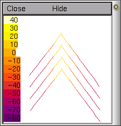 Each time we create a new section and
connect it to others, NEURON places the
section in a 3-D space and assigns an X, Y and Z coordinate to
each end of the section. When creating more than one neuron, as
we have above, each neuron is given a different Z coordinate
for all of its sections. The X and Y coordinates of each neuron
are determined by how the individual sections are connected.
This makes viewing the neurons difficult since they are not
arranged how we would normally think of them. To see the
default position of neurons, open a space plot (under the
Graph menu) and 3D rotate the neurons (see part B for instructions on space plots); an
example is shown on the left.
Each time we create a new section and
connect it to others, NEURON places the
section in a 3-D space and assigns an X, Y and Z coordinate to
each end of the section. When creating more than one neuron, as
we have above, each neuron is given a different Z coordinate
for all of its sections. The X and Y coordinates of each neuron
are determined by how the individual sections are connected.
This makes viewing the neurons difficult since they are not
arranged how we would normally think of them. To see the
default position of neurons, open a space plot (under the
Graph menu) and 3D rotate the neurons (see part B for instructions on space plots); an
example is shown on the left.
Fortunately, NEURON provides a way to
reposition each section in the 3-D space. We can use two
functions to reposition each section: pt3dclear() and pt3dadd(). The
first, pt3dclear(), will erase any 3-D
positioning information associated with the section. The
second, pt3dadd(), takes four arguments
(X, Y, Z, and diam) and will add a new coordinate to the
section. Usually there are coordinates for each end of the
section which can be set by making two calls to
pt3dadd()--once for the "0" end of the section and
once for the "1" end of the section.
As you may be able to tell, there can be a lot of
information to enter for each neuron, particularly for complex
neuronal morphology where there are a large number of sections.
There are a number of ways to set up this information. For
example, neuron and section positions may be randomly placed
using built in random distributions, or the tree portions may
explicitly follow experimentally derived anatomical
measurements, and these may be read from a file.
We will now dramatically enhance our neuron template, by
reintroducing a more complete dendritic tree morphology read
from two files (one for each of the two trees). The code for
this is in the sthC2.hoc hoc
file. The system is very similar to the neurons we have created
so far (using the template defined above), except now, rather
than two dendrites (each being a section) we have two trees,
containing 23 and 11 dendritic branches respectively (these
values are defined from the full tree morphology illustrated in
part B). The tree properties are specified in the text files
treeA.dat and treeB.dat. The files can
have virtually any format, as how the information is read is
specified in our template. These example files contain as their
first line the number of sections in the tree. Each following
line has the following format:
branch-num child1 child2 diam
L X Y Z X Y Z
where branch-num is the reference number of the
branch (starting at 1), child1 and child2 are the
daughter branches reference numbers (0 if there is no
daughter), diam and L are the branch diameter and
length respectively, and the two 3D coordinate points are the
branches 3D position (start and end points of the
cylinder).
Our STh neuron template begins in a very similar manner to
the example above:
begintemplate SThcell
public soma, treeA, treeB

create soma, treeA[1], treeB[1]
objectvar f

proc init() {local i, me, child1, child2

    create soma

    soma {
      nseg = 1
      diam = 18.8
      L = 18.8
      Ra = 123.0
      insert hh
      gnabar_hh=0.25
      gl_hh = .0001666
      el_hh = -60.0
    }
We have made the soma, treeA and
treeB public, so, for example, we could place
electrodes anywhere along the dendritic trees. We have also
created a new objectvar f used to reference
the files. The soma definition is the same as we have
previously used.
Note, we have not yet created our trees. Unlike the previous
example, we no longer know the number of sections in the trees
as this is now specified in the tree files (in their first
lines).
However, notice that we have already created tree section
arrays of length one just before the init() procedure.
Because NEURON dynamically interprets the
commands, each section and object variable must be declared
before they are used. This means that in order for NEURON to know how to interpret commands about a
section, it must be declared before the code that accesses it
is interpreted by NEURON. For example, the
following code would return an error since treeA is
not created, in this example as an array of 2 sections, before
the procedure is interpreted:
begintemplate SThcell
public soma
create soma

proc init() {

    create soma, treeA[2]

    treeA[0] {
      nseg = 5
      diam = 3.18

...
Even though the create treeA[2] command exists,
treeA is not created until the procedure init
is called. Thus, when NEURON
interprets any treeA[i] code, it does not yet have any
section of object named treeA, so it returns an error.
To correct this we need to create the treeA and
treeB sections outside of the
init()procedure. Now we have a different problem: we
do not know the correct number of treeA or
treeB sections to create, since this information is
read from the files. NEURON solves this
problem by allowing you to redeclare a section or an array of
sections inside a procedure. For this simple example, we need
to create an array of treeA and treeB
sections before the procedure init(). The number of
elements in the array does not matter, since we will re-create
the array inside the procedure.
In general, the two rules we need to follow are:
- If a section or object is referenced inside a procedure,
create or declare it before the procedure in which it is
used.
- When creating or declaring an array of sections or
objects that will be recreated or redeclared inside a
procedure, create or declare an array of length 1 before the
procedure in which the sections or objects are recreated or
redeclared.
To access a file, we need to create a new file object. This
is done in a similar manner to creating other objects (for
example the IClamp in part A):
  f = new File()
  f.ropen("treeA.dat")
The first line creates the file object, the second uses the
file object function ropen() to open the
file treeA.dat to read. To read a single value from
the file we will use the function scanvar(). Thus we can read the correct number of
sections in our tree from the first line of the file and then
create them by redefining our tree sections:
   ndendA = f.scanvar()
   create treeA[ndendA]
Now we can continue to use f.scanvar()
to read the rest of our file. For example, if the next line of
our file treeA.dat was:
1 2 3 3.180 10.000 0.000 0.000 0.000 18.092 -0.346 4.932
then the second call to f.scanvar()
returns the value 1, the third use of f.scanvar() returns the value 2, the fourth
returns 3 and the fifth returns 3.180 etc. Thus
we can define our dendritic tree treeA using the
following code:
    for i = 0,ndendA-1 {
      me = f.scanvar() - 1
      child1 = f.scanvar() - 1
      child2 = f.scanvar() - 1

      treeA[me] {
        nseg = 1
        diam = f.scanvar()
        L = f.scanvar()
        Ra = 123
        // initialise and clear the 3D information
        pt3dclear()
        pt3dadd(f.scanvar(),f.scanvar(),f.scanvar(),diam)
        pt3dadd(f.scanvar(),f.scanvar(),f.scanvar(),diam)
        insert pas
        g_pas = .0001666
        e_pas = -60.0

        if (child1 >= 0) {
          connect treeA[child1](0), 1
        }
        if (child2 >= 0) {
          connect treeA[child2](0), 1
        }
      }
    }
 This is a loop creating
each section/branch of the tree as defined by the file. The
local variable me is the first value read from the file,
and is the reference for this branch. As we know, arrays start
at 0, however, our file references start at 1, so the variable
me is defined as f.scanvar() - 1. Similarly the
references for child1 and child2 branches have 1
subtracted. The branch diameter diam and length L
are directly read from the file. Finally all the 3D position
information is read from the file and the branch sections are
connected up to form the tree.
This is a loop creating
each section/branch of the tree as defined by the file. The
local variable me is the first value read from the file,
and is the reference for this branch. As we know, arrays start
at 0, however, our file references start at 1, so the variable
me is defined as f.scanvar() - 1. Similarly the
references for child1 and child2 branches have 1
subtracted. The branch diameter diam and length L
are directly read from the file. Finally all the 3D position
information is read from the file and the branch sections are
connected up to form the tree.
The loop repeats this setup for each branch/section (note
the number of tree sections for each tree is passed as the two
parameters to the template). The second tree (treeB)
is done in a very similar manner. To complete our template,
after both trees have been read in from the files, we must
connect the trees to the soma:
    // Connect things to the soma
    connect treeA[0](0), soma(1)
    connect treeB[0](0), soma(0)
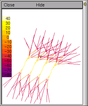
The final four neurons, each with a full dendritic tree
morphology is shown here in a shape plot. This form of shape
plot shows the voltage of the sections as a hot scale (hot
colours mean high voltage, cool colours low voltage as
indicated in the scale).
Note, in this example, each branch/section only has one
segment, independent of how long the branch may be. You may
want to increase the number of segments for a higher spatial
resolution (see part B).
Connecting the neurons together -
NetCon
We have not yet connected our neurons together. Currently,
they are operating as four independent subthalamic neurons,
each with an electrode placed in the soma. The modern form of
connecting neurons together is in an event based simulation
model. Events are usually things like action potentials,
as it is the events (rather than, for example, the specific
voltage levels) that we need to pass or communicate between
neurons. By using an event based model, we can dramatically
reduce the amount of inter-neuron communication. This is
important in simulation time optimisation and in simulations on
parallel machines.
First we must add an additional public object variable to
the neuron template. The new object variable will refer to a
list that will hold an arbitrary number of NetCon objects. A
NetCon object is an object associated with a particular source
of events (usually a soma, where action potentials produce the
binary events). So, we now begin our subthalamic neuron
template with the following:
begintemplate SThcell
public soma, treeA, treeB, nclist

create soma, treeA[1], treeB[1]
objectvar f, nclist

proc init() {local i, me, child1, child2

    create soma

    nclist = new List()
The only thing we have changed is to add a object variable
nclist, make it public, and in the init()
procedure, associate it with a new List.
In NEURON a List is an
object that holds a list of other objects. The advantage of a
list is that we don't have to specify in advance how big it
will grow, as we do with an array. We will see later how to add
items to a list and change their values.
Let's now modify the code so only one neuron is being
stimulated by an electrode. Choose SThcells[1] to have
an electrode placed in the soma to produce action potentials
between 100 and 200 ms. Having done Parts A and B of the
tutorial, you should be able to modify the code and remove the
electrodes from the other neurons.
Now, from 100 to 200 ms, neuron SThcells[1]
will be generating action potentials. In our first connection
example, we only want to connect this neuron to
SThcells[0] and observe the EPSPs (Excitatory Post
Synaptic Potentials) at the soma of neuron 0.
We must first create some synaptic objects. Like
IClamps, discussed in part A, a synapse is simply an
object that can be positioned anywhere on a neuron. For
example, at the end of our current code we can define a new
array of objects for our synapses. Here, we have a maximum of
10 synapses:
maxsyn = 10
objectvar syn[maxsyn]
We will use the built in synaptic type ExpSyn, which is a synapse whose conductance
instantaneously rises on receiving a spike and then
exponentially decays. We position the synapse when it is
created (in the same manner to IClamps) i.e. refer to
a section of a neuron where we wish the synapse to be located
and create the synapse there:
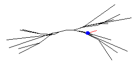
SThcells[0].treeA[7] syn[0] = new ExpSyn(0)
In this example, we have created an ExpSyn synapse
(syn[0]) positioned at the proximal end of
treeA dendritic branch 7 on subthalamic neuron 0
(marked here by the small blue square):
Now we must define the source of events for this synapse.
This will be the action potentials generated at the soma of
SThcells[1]. As SThcells[0] receives the
events (i.e. this is the neuron where the synapse is) we must
append a new NetCon object to the
nclist of this neuron. To create a new NetCon
object, we use the command format:
new NetCon(&source_v, synapse, threshold,
delay, weight)
where source_v is the source voltage (in our
case the voltage from SThcells[1].soma),
synapse is the object variable that refers to
the synaptic object receiving the events (in our case
syn[0]), threshold is the threshold
which the voltage must reach for it to be considered that an
action potential has occurred, delay is the
connection delay, and weight is the connection
weight strength at the synapse. So to connect
SThcells[1] to the proximal end of treeA dendritic
branch 7 on subthalamic neuron SThcells[0] we add the
command:
SThcells[1].soma SThcells[0].nclist.append(new
                NetCon(&v(1), syn[0], -20, 1, 0.5))
First this command accesses SThcells[1].soma, then
the nclist of cell SThcells[0] has a new NetCon object appended. This NetCon object has a source voltage of
SThcells[1].soma.v(1) (note, as we have accessed
SThcells[1].soma in the command above, we need only
use the short variable v(1)). The NetCon object applies to syn[0] which we
have already attached to SThcells[0].treeA[7] (see
above). Our threshold for action potentials is -20mV, our delay
1ms, and our synaptic weight 0.5.
If we run the simulation and plot the voltage at
SThcells[0].soma we see EPSPs resulting from the
action potentials of neuron SThcells[1]:
![SThcells[0].soma.v(0.5)](sthcells0.gif)
![SThcells[1].soma.v(0.5)](sthcells1.gif)
Dealing with lists
How do we change the weight, threshold and delay of our NetCon objects? If we had declared an objectvar called nc, we would have
been able to refer to nc.weight, nc,threshold
and nc.delay. However, our NetCon
objects are embedded in a list, so we can't.
The solution is a group of commands to deal with lists. As
mentioned above, the command
nclist.append(obj)
appends the object specified by the object variable
obj to the list nclist. We can use the
command
nclist.count()
to return the number of items in the list nclist.
The command
nclist.object(i)
returns the object at index i in the list
nclist.
We can put these commands together to change properties of
the connections. For example:
for i = 0, SThcells[0].nclist.count()-1 {
    SThcells[0].nclist.object(i).weight = 0.6
}
will change all of the weights onto SThcells[0] to
0.6.
Try playing with the connection parameters (delay, threshold
and weight) and then connect more of the neurons together using
more of the synaptic objects (but remember we have only created
10 objectvars to refer to synaptic objects in this
example; feel free to add more by increasing the
maxsyn parameter).
In part D of this tutorial, we will
make the neurons much more characteristic of subthalamic
nucleus neurons by building our own channel types using NMODL.
Andrew Gillies (andrew@anc.ed.ac.uk)
David Sterratt (dcs@anc.ed.ac.uk)
based on the tutorials by Kevin E. Martin
with the assistance of Ted Carnevale and Michael Hines
Last modified on