6.4.12 Single-Depot VRPWe shall examine next the following version of the vehicle routing problem. Let there be n demand points in a given area, each demanding a quantity of weight Qi (i = 1, 2, . . . , n) of goods to be delivered to it (goods are assumed indistinguishable but for their weight). The goods in question are stored at a depot, D, where a fleet of vehicles is also stationed. Vehicles have identical maximum weight capacities and maximum routetime (or distance) constraints. They must all start and finish their routes at the depot, D. The problem is to obtain a set of delivery routes from the depot, D, to the various demand points to minimize the total distance covered by the entire fleet. It is assumed that the weights Qi (i = i , . . . , n) of the quantities demanded are less than the maximum weight capacity of the vehicles and we require that the whole quantity Qi demanded at a given point i be delivered by a single vehicle (i.e., we do not allow for the possibility that one third, say, of Qi will be delivered by one vehicle and the remaining two thirds by another). Obviously, the words "supply" and "quantity supplied" can be substituted for "demand" and "quantity demanded," in which case the depot becomes a collection point. Thus, the VRP applies equally well to solid waste collection from a specific set of points and to parcel delivery to a set of points. A notable recent application, for instance, has been in routing of newspaper distribution vehicles delivering editions of a well-known newspaper to newsstands in an urban area [GOLD 77]. We also note that in specific applications of the VRP, either the maximum weight or the maximum route-time constraints may be relaxed. However, both usually play a role. For instance, in the newspaper delivery problem just mentioned, one constraint, in addition to the maximum number of newspapers that a vehicle can carry, was that all deliveries to newsstands must be made within an hour of press time. When neither constraint applies, the VRP reduces to a traveling salesman problem: if the objective is simply to minimize total distance, it is a 1-TSP [from (6.10)]; if the number of vehicles to be used is specified, it is a m-TSP. It can thus be seen that TSP's can be viewed as special cases of VRP's. By inference, VRP's can be expected to be more difficult than TSP's as far as optimum solutions are concerned. Indeed, although several versions of VRP's have been formulated as mathematical programming problems by various investigators, the largest vehicle routing problems of any complexity that have been solved exactly reportedly involved less than 30 delivery points [CHRI 74]. By contrast, the heuristic approaches that we shall describe next can be used even with thousands of delivery points. Heuristics for the single-depot VRP. By far the
best-known approach to the VRP problem is the "savings" algorithm of
Clarke and Wright. Its basic idea is very simple. Consider a depot D and
n demand points. Suppose that initially the solution to the VRP consists
of using n vehides and dispatching one vehicle to each one of the n demand
points. The total tour length of this solution is, obviously,
2 If now we use a single vehicle to serve two points, say i and j, on a
single trip, the total distance traveled is reduced by the amount
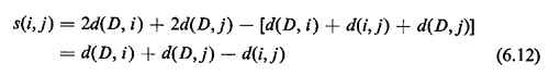
The quantity s(i, j) is known as the "savings" resulting from combining points i and j into a single tour. The larger s(i, j) is, the more desirable it becomes to combine i and j in a single tour. However, i and j cannot be combined if in doing so the resulting tour violates one or more of the constraints of the VRP. The algorithm can now be described as follows. Clark>Wright Savings Algorithm (Algorithm 6.7)
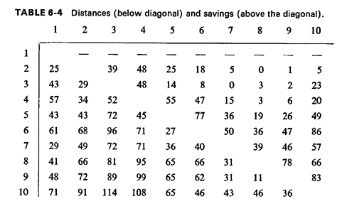
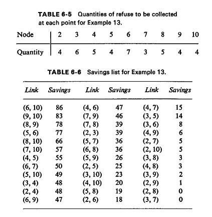
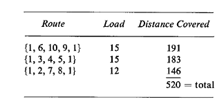
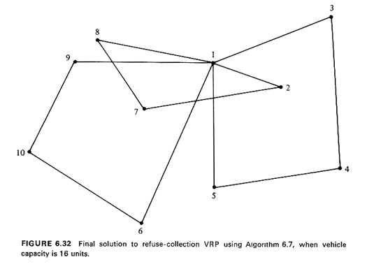
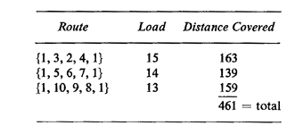
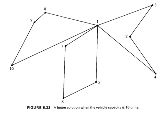
Example 13: Refuse-Collection, Revisited 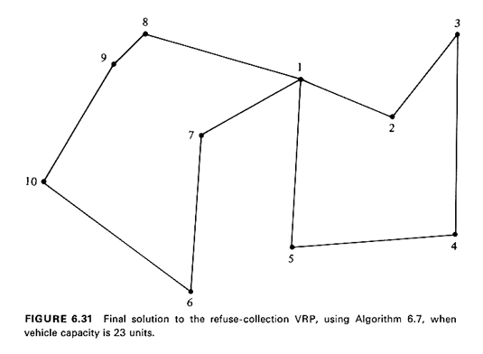
As the reader may have already surmised, the Clarke-Wright algorithm can be programmed to run very efficiently and, since it involves very simple manipulations of the data set, it can be used with large problems. Because nodes are added to routes one or two at a time, an additional advantage of the algorithm is that it is possible to check whether each addition would violate any set of constraints, even when that set is quite complicated. For instance, besides the constraints on maximum capacity and maximum distance, other constraints might be included, such as a maximum number of points that any vehicle may visit. On the other hand, there is no guarantee that the solution provided by such a naive algorithm will be anywhere close to the optimum. While experience has shown that the algorithm performs quite well most of the time, it is possible to devise "pathological" cases for which the Clarke-Wright solutions are very poor indeed. However, it is often possible to improve considerably, by inspection, a set of VRP tours produced by the savings algorithm. In fact, a powerful interactive "man-machine" approach has been developed for that purpose [KROL 72. In this approach, a computer "suggests" a solution using the savings algorithm and projects that solution on a television screen. The human operator then attempts to improve on this solution using his/her knowledge of the problem as well as such geometrical properties of good tours as those we have already discussed for the Euclidean TSP (Section 6.4.8). The operator, using a light pen, suggests these improvements to the computer, which, in turn, comes up with a new solution to the VRP; and so on.
Several alternatives to the Clarke-Wright algorithm have been proposed. One that seems to produce good solutions to VRP,s can be summarized as follows [GILL 74b]. Sweep Algorithm for the VRP (Algorithm 6.8) Assume that polar coordinates are available for all points to be visited by the vehicles (the depot, for instance, might be used as the origin in the coordinate system). The points then can be ordered in terms of increasing angle by sweeping (clockwise or counterclockwise) a ray initially drawn from the depot to some arbitrary point--known as the seed point. Routes are then drawn up by adding demand points to a route as these demand points are swept: beginning at the seed (whose angle can be set to 0), points are included in a route as they are swept, until the load capacity of a vehicle precludes addition of the next point swept to the current route. That point then becomes the seed for the next route and the process is completed when all points have been swept (i.e., included in a route). Once the points that form each route are available, a TSP algorithm can be used to determine the order of point traversal for each individual route. Thus, the sweep algorithm is a good example of the "cluster first, route second" approach.
The major disadvantage of the sweep algorithm is that it does not generate the vehicle tours as it processes the nodes. This is done only after the nodes that constitute each tour have been specified and thus becomes a time-consuming procedure. In addition, whenever there are constraints on the maximum tour lengths as well, some clusters may prove to lead to tours that are unacceptably long. Finally, the algorithm requires Euclidean distances and satisfaction of the triangular inequality throughout. In general, the Clarke-Wright algorithm seems to enjoy an advantage in terms of both efficiency and flexibility over other available VRP algorithms and has been used extensively. The method has been programmed as the VSPX (Vehicle Scheduling Program) package by IBM and is thus available commercially. The algorithm can be rendered even more powerful through a simple modification that forces the algorithm to generate several alternative solutions and through careful organization and storage of the information it utilizes [GOLD 76]. |
 d(D, i).