|
|
|
| Thermodynamics and Propulsion | |
|
Next: 7.6 Summary and Conclusions Up: 7. Entropy on the Previous: 7.4 The Statistical Definition Contents Index 7.5 Numerical Example of the Approach to the Equilibrium Distribution
Reynolds and Perkins give a numerical example which illustrates the
above concepts and also the tendency of a closed isolated system to
tend to equilibrium. The starting point is a system in an initial
microscopic state that is not an equilibrium distribution. We expect
the system will change quantum state, with disorder, randomness
growing until they reach the equilibrium values. The specific system
to be studied is composed of 10 particles
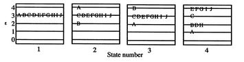
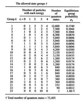
For ten particles, 4 energy states, and a total energy of 30, there are 72,403 possible quantum states (4 states are indicated in Figure 7.1). However, there are only 23 possible distributions in terms of the number of particles having a given energy as shown in Figure 7.2. For example, states 2 and 3 in Figure 7.1 are two different quantum states, but they represent the same group (22) in Figure 7.2. The allowed state groups
If the quantum-state probabilities are equal, each quantum state has
a probability of 1/72,403. The probabilities of each group are thus
directly proportional to the number of quantum states in this group.
For instance, group 22 has 90 quantum states, so its probability is
If the system is initially in state 1 of
Figure 7.1, it is in group 23 of
Figure 7.2. For each of the 45
pairs, there are two interactions that take the system to group 22,
and one that leaves the system unchanged. (For interactions between
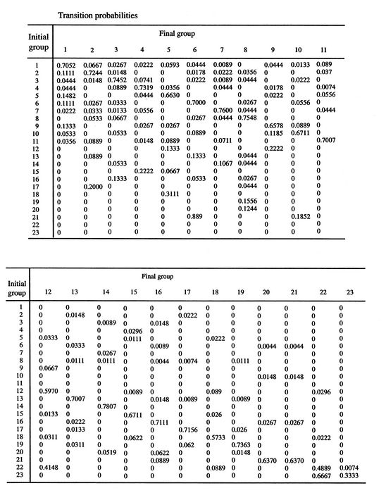
For the other groups, the transitions are more complicated, but can
be found numerically, with the results shown in
Figure 7.3. The numerical experiments
were carried out with the system initially in state 23 and with
successive interactions chosen randomly in accordance with the
transition probabilities of
Figure 7.3. The experiment was
repeated 10,000 times, with a different group history traced out
each time and, again, the system energy maintained at 30. The
fraction of the experiments in which each group occurred at time
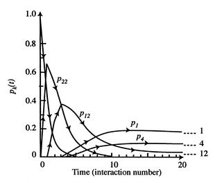
Figure 7.4 shows the evolution
of some of the
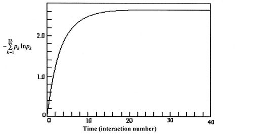
The computed entropy is given in Figure 7.5 as a function of time. It increases to the equilibrium value with the same sort of behavior as the probability distribution. The interactions allow the system to change groups. The transition probabilities are large for groups with high equilibrium probabilities.
There is one additional aspect of the behavior that is brought out
in the text. This is the difference in overall probabilities between
the order of transitions. The probability of a transition sequence
is the product of the individual step transition probabilities. The
transition 23-22-12-9-1 thus has the probability:
Next: 7.6 Summary and Conclusions Up: 7. Entropy on the Previous: 7.4 The Statistical Definition Contents Index |