Burt Rutan's White Knight and SpaceShip One, Photo Courtesy of Scaled Composites
Thermodynamics and Propulsion
Subsections

13.3 Aircraft Range: the Breguet Range Equation

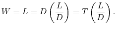
Consider an aircraft in steady, level flight, with weight $ W$ , as shown in Figure 13.1. The rate of change of the gross weight of the vehicle is equal to the fuel weight flow:

$\displaystyle -\frac{dW}{dt}=g\dot{m}_f = \frac{T}{I_{sp}}.$

For steady, level flight, $ T = D$ , $ L = W$ , or

$\displaystyle W=L=D\left(\frac{L}{D}\right)=T\left(\frac{L}{D}\right).$

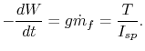
The rate of change of aircraft gross weight is thus
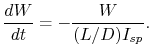
$\displaystyle \frac{dW}{dt} =-\frac{W}{(L/D)I_{sp}}.$

Suppose $ L/D$ and $ I_{sp}$ remain constant along the flight path:

$\displaystyle \frac{dW}{W} = -\frac{dt}{(L/D)I_{sp}}.$

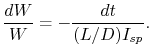
We can integrate this equation for the change in aircraft weight to yield a relation between the weight change and the time of flight:
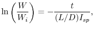
$\displaystyle \ln\left(\frac{W}{W_i}\right)=-\frac{t}{(L/D)I_{sp}},$

where $ W_i$ is the initial weight. If $ W_f$ is the final weight of vehicle and $ t_\textrm{initial}=0$ , the relation between vehicle parameters and flight time, $ t_f$ , is

$\displaystyle \frac{L}{D}I_{sp} \ln\left(\frac{W_i}{W_f}\right)=t_f.$

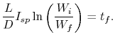
The range is the flight time multiplied by the flight speed, or,

$\displaystyle \textrm{Range } = V t_f = V \times \underbrace{\left(\frac{L}{D}\...
...imes \underbrace{\ln\left(\frac{W_i}{W_f}\right)}_\textrm{structural designer}.$

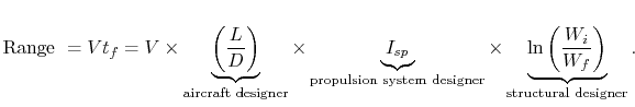
The above equation is known as the Breguet range equation. It shows the influence of aircraft, propulsion system, and structural design parameters.

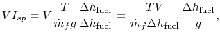
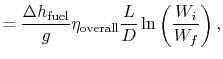
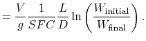
13.3.1 Relation of overall efficiency, $ I_{sp}$ , and thermal efficiency

Suppose $ \Delta h_\textrm{fuel}$ is the heating value (``heat of combustion'') of the fuel (i.e., the energy per unit of fuel mass), in J/kg. The rate of energy release is $ \dot{m}_f\Delta h_\textrm{fuel}$ , so

$\displaystyle V I_{sp} = V \frac{T}{\dot{m}_f g}\frac{\Delta h_\textrm{fuel}}{\...
...}
=\frac{T V}{\dot{m}_f\Delta h_\textrm{fuel}}\frac{\Delta
h_\textrm{fuel}}{g},$

and

$\displaystyle \frac{T V}{\dot{m}_f\Delta h_\textrm{fuel}}=
\frac{\textrm{Thrust...
...gy}}
= \eta_\textrm{overall}\; \textrm{(overall propulsion system
efficiency)}.$

Thus

$\displaystyle \eta_\textrm{overall} = \frac{g}{\Delta h_\textrm{fuel}}V I_{sp}$

and

$\displaystyle \textrm{Range }$ $\displaystyle = \frac{\Delta h_\textrm{fuel}}{g}\eta_\textrm{overall}\frac{L}{D}\ln\left(\frac{W_i}{W_f}\right),$    

or


$\displaystyle \textrm{Range }$ $\displaystyle = \frac{V}{g}\frac{1}{SFC}\frac{L}{D}\ln\left(\frac{W_{\textrm{initial}}}{W_{\textrm{final}}}\right).$    

Keep in mind that, in general,

$\displaystyle \eta_\textrm{overall} = \eta_\textrm{thermal} \eta_\textrm{propulsive} \eta_\textrm{combustion}.$


13.3.2 The Propulsion Energy Conversion Chain

The above concepts are depicted in Figure 13.4 as parts of the propulsion energy conversion train mentioned in Part I, which shows the process from chemical energy contained in the fuel to energy useful to the vehicle.

Figure 13.4: The propulsion energy conversion chain from Part I
Image fig5PropulsionEnergyConversionChain_web

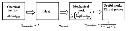
The combustion efficiency is near unity unless conditions are far off design. We can therefore regard the two main drivers as the thermal and propulsive13.1 efficiencies. The evolution of the overall efficiency of aircraft engines in terms of these quantities was shown in Figure 11.8.

UnifiedTP