1.2
Charge and Current Densities

In Maxwell's day, it was not known that charges are not infinitely divisible but occur in elementary units of 1.6 x 10^-19 coulomb, the charge of an electron. Hence, Maxwell's macroscopic theory deals with continuous charge distributions. This is an adequate description for fields of engineering interest that are produced by aggregates of large numbers of elementary charges. These aggregates produce charge distributions that are described conveniently in terms of a charge per unit volume, a charge density .

Pick an incremental volume and determine the net charge within. Then

is the charge density at the position r when the time is t. The units of are coulomb/meter³. The volume V is chosen small as compared to the dimensions of the system of interest, but large enough so as to contain many elementary charges. The charge density is treated as a continuous function of position. The "graininess" of the charge distribution is ignored in such a "macroscopic" treatment.

Fundamentally, current is charge transport and connotes the time rate of change of charge. Current density is a directed current per unit area and hence measured in (coulomb/second)/meter². A charge density moving at a velocity v implies a rate of charge transport per unit area, a current density J, given by

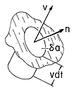
Figure 1.2.1 Current density J passing through surface having a normal n

One way to envision this relation is shown in Fig. 1.2.1, where a charge density having velocity v traverses a differential area a. The area element has a unit normal n, so that a differential area vector can be defined as a = n a. The charge that passes during a differential time t is equal to the total charge contained in the volume v a dt. Therefore,

Divided by dt, we expect (3) to take the form J a, so it follows that the current density is related to the charge density by (2).

The velocity v is the velocity of the charge. Just how the charge is set into motion depends on the physical situation. The charge might be suspended in or on an insulating material which is itself in motion. In that case, the velocity would also be that of the material. More likely, it is the result of applying an electric field to a conductor, as considered in Chap. 7. For charged particles moving in vacuum, it might result from motions represented by the laws of Newton and Lorentz, as illustrated in the examples in Sec.1.1. This is the case in the following example.

Example 1.2.1. Charge and Current Densities in a Vacuum Diode

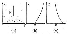
Consider the charge and current densities for electrons being emitted with initial velocity v from a "cathode" in the plane x = 0, as shown in Fig. 1.2.2a.

---

¹ Here we picture the field variables E_x, v_x, and as though they were positive. For electrons, < 0, and to make v_x > 0, we must have E_x < 0.

---

Figure 1.2.2 Charge injected at the lower boundary is accelerated upward by an electric field. Vertical distributions of (a) field intensity, (b) velocity and (c) charge density.

Electrons are continuously injected. As in Example 1.1.1, where the motions of the individual electrons are considered, the electric field is assumed to be uniform. In the next section, it is recognized that charge is the source of the electric field. Here it is assumed that the charge used to impose the uniform field is much greater than the "space charge" associated with the electrons. This is justified in the limit of a low electron current. Any one of the electrons has a position and velocity given by (1.1.7) and (1.1.8). If each is injected with the same initial velocity, the charge and current densities in any given plane x = constant would be expected to be independent of time. Moreover, the current passing any x-plane should be the same as that passing any other such plane. That is, in the steady state, the current density is independent of not only time but x as well. Thus, it is possible to write

where J_o is a given current density.

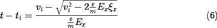
The following steps illustrate how this condition of current continuity makes it possible to shift from a description of the particle motions described with time as the independent variable to one in which coordinates (x, y, z) (or for short r) are the independent coordinates. The relation between time and position for the electron described by (1.1.7) takes the form of a quadratic in (t - t_i)

This can be solved to give the elapsed time for a particle to reach the position _x. Note that of the two possible solutions to (5), the one selected satisfies the condition that when t = t_i, _x = 0.

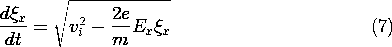
With the benefit of this expression, the velocity given by (1.1.8) is written as

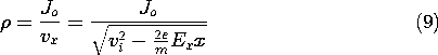
Now we make a shift in viewpoint. On the left in (7) is the velocity v_x of the particle that is at the location _x = x. Substitution of variables then gives

so that x becomes the independent variable used to express the dependent variable v_x. It follows from this expression and (4) that the charge density

is also expressed as a function of x. In the plots shown in Fig. 1.2.2, it is assumed that E_x < 0, so that the electrons have velocities that increase monotonically with x. As should be expected, the charge density decreases with x because as they speed up, the electrons thin out to keep the current density constant.