12.2
Electrodynamic Fields of Source Singularities

Given the response to an elemental source, the fields associated with an arbitrary distribution of sources can be found by superposition. This approach will be formalized in the next section and can be utilized for determining the radiation patterns of many antenna arrays. The fields resulting from this superposition principle form a particular solution that can be combined with solutions to the homogeneous wave equation to satisfy the boundary conditions imposed by perfectly conducting boundaries.

We begin by identifying the potential associated with a time varying point charge q(t). In a closed system, where the net charge is invariant, an increase in charge at one point must be compensated by a decrease in charge elsewhere. Thus, as we shall see in identifying the fields of an electric dipole, physically meaningful fields are the superposition of those produced by at least two point charges of opposite sign. Conservation of charge further requires that this shift in the distribution of net charge from one region to another be accounted for by a current. This current is the source term in the inhomogeneous wave equation for the vector potential.

Potential of a Point Charge

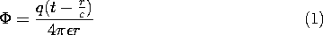
Consider the potential predicted by the inhomogeneous wave equation, (12.1.10), for a time varying point charge q(t) located at the origin of the spherical coordinate system shown in Fig. 12.2.1.

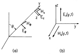
Figure 12.2.1 A point charge located at the origin of a spherical coordinate system.

By definition, is zero everywhere except at the origin, where it is singular.

In the immediate neighborhood of the origin, we should expect that the potential varies so rapidly with r that the Laplacian would dominate the second time derivative in the inhomogeneous wave equation, (12.1.10). Then, in the vicinity of the origin, we should expect the potential for a point charge to be the same as for Poisson's equation, namely q(t)/(4 r) (4.4.1). From Sec. 3.1, we have a hint as to how the combined effects of the magnetic induction and electric displacement current represented by the second time derivative in the inhomogeneous wave-equation, (12.1.10), should affect this potential. We can expect that the response at a radial position r will be delayed by the time required for an electromagnetic wave to reach that position from the origin. For a wave propagating at the velocity c, this time is r/c. Thus, we make the educated guess that the solution to (12.1.10) for a point charge at the origin is

where c = 1/. According to (1), given that the time dependence of the point charge is q(t), the potential at radius r is given by the familiar potential for a point charge, provided that t (t - r/c).

Verification that of (1) is a solution to the inhomogeneous wave equation (12.1.10) takes two steps. First, the expression is substituted into the homogeneous wave equation [(12.1.10) with no source] to see that it is satisfied everywhere except at the origin. In carrying out this step, note that is a function of the spherical radial coordinate r alone. Thus, ² is simply r^-2 (r² / r)/ r. This operation gives the same result as the operation r^{-1 2} (r )/ r². Thus, evaluated using the potential of (1), the terms on the left in the inhomogeneous wave equation, (12.1.10), become

for r 0. In carrying out this evaluation, note that q/ r = - q^' /c and q/ t = q^' where the prime indicates a derivative with respect to the argument. Thus, the homogeneous wave equation is satisfied everywhere except at the origin.

In the second step, we confirm that (1) is the dynamic potential of a point charge. We integrate the inhomogeneous wave equation in the neighborhood of r = 0, (12.1.10), over a small spherical volume of radius r centered on the origin.

The Laplacian has been written in terms of its definition in anticipation of using Gauss' theorem to convert the first integral to one over the surface at r. In the limit where r is small, the integration of the second time derivative term gives no contribution.

Integration of the first term on the left in (3) is familiar from Chap. 4, because Gauss' theorem converts the volume integration to one over the enclosing surface and we therefore have

In the limit where r 0, the integral on the right in (3) gives q/. Thus, it reduces to the same expression obtained using (1) to evaluate the left-hand side of (3). We conclude that (1) is indeed the solution to the inhomogeneous wave equation for a point charge at the origin.

Electric Dipole Field

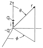
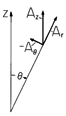
An electric dipole consists of a pair of charges q(t) separated by the distance d, as shown in Fig. 12.2.2. As one charge increases in magnitude at the expense of the other, there is an elemental current i(t) directed between the two along the z axis. Charge conservation requires that

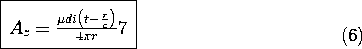
This current can be pictured as a singularity in the distribution of the current density J_z. In fact, the role played by / as the source of on the right in (12.1.10) is played by J_z in determining A_z in (12.1.8). Just as q can be regarded as the integral of the charge density over the elemental volume occupied by that charge density, id is J_z first integrated over the cross-sectional area in the x - y plane of the current tube joining the charges (to give i) and then integrated over the length d of the tube. Thus, we exploit the analogy between the z component of the vector inhomogeneous wave equation for A_z and that for , (12.1.8) and (12.1.10), to write the vector potential associated with an incremental current element at the origin. The solution to (12.1.8) is the same as that to (12.1.10) with q/ id.

Figure 12.2.2 A dynamic dipole in which the time-variation of the charge is accounted for by the elemental current i(t).

Remember that r is a spherical coordinate, so it is best to convert this expression into spherical coordinates. Figure 12.2.3 shows that

Thus, in spherical coordinates, (7) becomes the vector potential for an electric dipole.

Figure 12.2.3 The z-directed potential is analyzed into its components in spherical coordinates.

The dipole scalar potential is the superposition of the potentials due to the individual charges, (5). The positive charge is located on the z axis at z = d, while the negative one is at the origin, so superposition gives

where, in a way familiar from Sec. 4.4, the distance from the point of observation to the charge at z = d is approximated by r - d cos . With q^' indicating a derivative with respect to the argument, expansion in a Taylor's series based on d cos r gives

and keeping terms that are linear in d results in the desired scalar potential for the electric dipole.

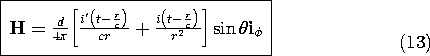
The vector potential (9) and scalar potential (12) obey (12.1.7), as can be confirmed by differentiation and use of the conservation law (6). We can now evaluate the magnetic and electric fields associated with these scalar and vector potentials. The magnetic field intensity follows by evaluating (12.1.1) using (9). [Remember that conservation of charge requires that q^' = i, in accordance with (6).]

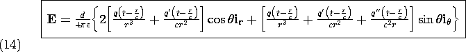
To find E, (12.1.3) is evaluated using (9) and (12).

As can be seen by comparing (14) to (4.4.10), in the limit where c , this electric field becomes the electric field found from the electroquasistatic dipole potential. Note that the quasistatic field is proportional to q (rather than its first or second temporal derivative) and decays as 1/r³. The first and second time derivatives of q are of order q/ and q/² respectively, where is the typical time interval within which q experiences an appreciable change. Thus, these time derivative terms are small compared to the quasistatic terms if r/c . What we have found gives substance to the arguments given for the EQS approximation in Sec. 3.3. That is, we have found that the quasistatic approximation is justified if the condition of (3.3.5) prevails.

The combination of electric displacement current and magnetic induction leading to the inhomogeneous wave equation has three dramatic effects on the dipole fields. First, the response at a location r is delayed⁴ by the transit time r/c. Second, the electric field is not only proportional to q(t - r/c), but also to q^' (t - r/c) and q^" (t - r/c). Third, the part of the electric field that is proportional to q^" decreases with radius in proportion to 1/r. Associated with this "far field" is a magnetic field, the first term in (13), that similarly decreases as 1/r. Together, these fields comprise an electromagnetic wave propagating radially outward from the dipole antenna.

⁴ In addition to the retarded response highlighted here, an "advanced" response, where t - r/c t + r/c, is also a solution to the inhomogeneous wave equation. Because it does not fit with our idea of causality, it is not used here.

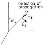
Note that these field components are orthogonal to each other and transverse to the radial direction of propagation, as shown in Fig. 12.2.4.

To appreciate the significance of the 1/r dependence of the fields in (15), consider the Poynting flux, (11.2.9), associated with these fields.

The power flow out through a spherical surface at the radius r follows from this expression as

Because the far fields of the dipole vary as 1/r, and hence the power flux density is proportional to 1/r², and because the area of the surface at r increases as r², we conclude that there is a net power flowing outward from the dipole at infinity. These far field components are called the radiation field.

Example 12.2.1. Turn-on Fields of an Electric Dipole

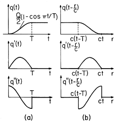
To help establish the physical significance of the electric dipole expressions for E and H, (13) and (14), consider the fields associated with charging an electric dipole through the transient shown in Fig. 12.2.5a. Over a period T, the charge increases from zero to Q with a continuous first derivative but a second derivative that suffers a finite discontinuity, as shown in the figure. Multiplied by appropriate factors of 1/r, 1/r², and 1/r³, the field distributions are made up of these three functions, with t replaced by t - r/c. Thus, at a given instant in time, the factors q(t - r/c), q^' (t - r/c), and q^"(t - r/c) have the radial distributions shown in Fig. 12.2.5b.

Figure 12.2.5 (a) Time dependence of the dipole charge q(t) as well as its first and second derivatives. (b) The radial dependence of the functions needed to evaluate the dipole fields resulting from the turn-on transient of (a) when t > T.

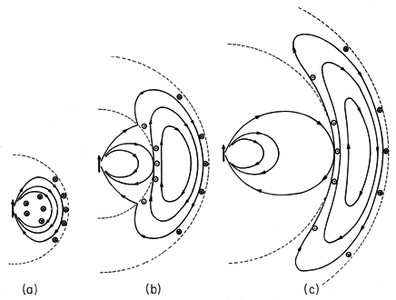
Figure 12.2.6 Electric fields (solid lines) and magnetic fields resulting from turning on an electric dipole in accordance with the temporal dependence indicated in Fig. 12.2.5. The fields are zero outside the wave front indicated by the outermost broken line. (a) For t < T, the entire field is in a transient state. (b) By the time t > T, the fields due to the transient are seen to be propagating outward between the expanding spherical surfaces at r = ct and r = c(t - T). Inside the latter surface, which is also indicated by a broken line, the fields are static. (c) At still later times, the propagating wave divorces itself from the dipole as the electric field generated by the magnetic induction, and the magnetic field generated by the displacement current, become self-sustaining.

The electric and magnetic fields are shown at three successive instants in time in Fig. 12.2.6. The transient part of the field is confined to an annular region with its outside radius at r = ct (the wave front) and inner radius at r = c(t - T). Inside this latter radius, the fields are static and composed only of those terms varying as 1/r³. Thus, when t = T (Fig. 12.2.6a), all of the field is transient, because the source has just reached a constant state. At the subsequent times t = 2T and t = 3T, the fields left behind by the outward propagating rear of the wave transient, the E field of a static electric dipole and H = 0, are as shown in Figs. 12.2.6b and 6c.

The flow of charges to the poles of the dipole produces an electromagnetic wave which reveals its identity once the annular region of the transient fields propagates out of the range of the near field. Note that the electric and magnetic fields shown in the outward propagating wave of Fig. 12.2.6c are mutually sustaining. In accordance with Faradays' law, the curl of E, which is directed and tends to be largest midway between the front and back of the wave, is balanced by a time rate of change of B which also has its largest value in the same region.

---

⁵In discerning a time rate of change implied by the figure, remember that the fields in the region of the spherical shell indicated by the two broken-line circles in Figs. 12.2.6b and 12.2.6c are propagating outward. Similarly, to satisfy Ampère's law, the -directed curl of H, which also peaks midway between the front and back of the wave, is balanced by a time rate of change of D that peaks in the same region.

---

It is instructive to review the discussion given in Sec. 3.3 of EQS and MQS approximations and their relation to electromagnetic waves. The electric dipole considered here in detail is the prototype system sketched in Fig. 3.3.1a. We have indeed found that if the condition of (3.3.5) is met, the EQS fields dominate. We should expect that if the current carried by the elemental loop of the prototype MQS system of Fig. 3.3.1b is a rapidly varying function of time, then the magnetic dipole (considered in the MQS limit in Sec. 8.3) also gives rise to a radiation field much like that discussed here. These fields are considered at the conclusion of this section.

Electric Dipole in the Sinusoidal Steady State

In the sections that follow, the fields of the electric dipole will be superimposed to obtain field patterns from antennae used at radio and microwave frequencies. In most of these practical situations, the field sources, q and i, are essentially in the sinusoidal steady state. In particular,

where is a complex number representing both the phase and amplitude of the current. Then, the general expression for the vector potential of the electric dipole, (7), becomes

Separation of the time dependence from the space dependence in solving the inhomogeneous wave equation is accomplished by the use of complex vector functions of space multiplied by exp j t. With the understanding that the time dependence is recovered by multiplying by exp (j t) and taking the real part, we will now deal with the complex amplitudes of the fields and drop the factor exp j t. Thus, (19) becomes

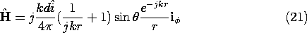
where the wave number k /c.

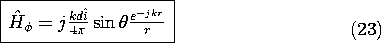
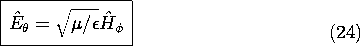
In terms of complex amplitudes, the magnetic and electric field intensities of the electric dipole follow from (13) and (14) as [by substituting q Re (/j ) exp (-jkr) exp (j t)]

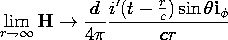
The far fields are given by terms with the 1/r dependence.

These fields, which are a special case of those pictured in Fig. 12.2.4, propagate radially outward. The far field pattern is a radial progression of the fields shown between the broken lines in Fig. 12.2.6c. (The response shown is the result of one half of a cycle.)

It follows from (23) and (24) that for a short dipole in the sinusoidal steady state, the power radiated per unit solid angle is

Equation (25) expresses the dependence of the radiated power on the direction ( , ), and can be called the radiation pattern. Often, only the functional dependence, ( , ) is identified with the "radiation pattern." In the case of the short electric dipole,

and the radiation pattern is as shown in Fig. 12.2.7.

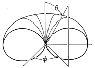
Figure 12.2.7 Radiation pattern of short electric dipole, shown in the range /2 < < 3 /2.

The Far-Field and Uniformly Polarized Plane Waves

For an observer far from the dipole, the variation of the field with respect to radius is more noticeable than that with respect to the angle . Further, if kr is large, the radial variation represented by exp (-jkr) dominates over the much weaker dependence due to the factor 1/r. This term makes the fields tend to repeat themselves every wavelength =2 /k. At frequencies of the order used for VHF television, the wavelength is on the order of a meter, while the station antenna is typically kilometers away. Thus, over the dimensions of a receiving antenna, the variations due to the factor 1/r and the variation in (23) and (24) are insignificant. By contrast, the receiving antenna has dimensions on the order of , and so the radial variation represented by exp (-jkr) is all-important. Far from the dipole, where spatial variations transverse to the radial direction of propagation are unimportant, and where the slow decay due to the 1/r term is negligible, the fields take the form of uniform plane waves. With the local spherical coordinates replaced by Cartesian coordinates, as shown in Fig. 12.2.8, the fields then take the form

That is, the fields depend only on y, which plays the role of r, and are directed transverse to y. Instead of the far fields given by (15), we have traveling-wave fields that, by virtue of their independence of the transverse coordinates, are called plane waves. To emphasize that the dipole has indeed launched a plane wave, in (15) we replace

and recognize that i^' = q^", (6), so that

The dynamics of such plane waves are described in Chap. 14. Note that the ratio of the magnitudes of E and H is the intrinsic impedance /. In free space, = _{o o} /_o 377 .

Figure 12.2.8 (a) Radiation field of electric dipole. (b) Cartesian representation in neighborhood of remote point.

Magnetic Dipole Field

Given the magnetic and electric fields of an electric dipole, (13) and (14), what are the electrodynamic fields of a magnetic dipole? We answer this question by exploiting a far-reaching property of Maxwell's equations, (12.0.7)-(12.0.10), as they apply where J_u = 0 and _u = 0. In such regions, Maxwell's equations are replicated by replacing H by -E, E by H, by , and by . It follows that because (13) and (14) are solutions to Maxwell's equations, then so are the fields.

Of course, q_m must now be interpreted as a source of divergence of H, i.e., a magnetic charge. Substitution shows that these fields do indeed satisfy Maxwell's equations with J = 0 and = 0, except at the origin. To discover the source singularity at the origin giving rise to these fields, they are examined in the limit where r 0. Observe that in the neighborhood of the origin, terms proportional to 1/r³ dominate H as given by (31). Close to the source, H takes the form of a magnetic dipole. This can be seen by a comparison of this near field to that given by (8.3.20) for a magnetic dipole.

With this identification of the source, (30) and (31) become

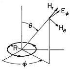
The small current loop of Fig. 12.2.9, which has a magnetic moment m = R² i, could be the source of the fields given by (33) and (34). If the current driving this loop were turned on in a manner analogous to that considered in Example 12.2.1, the field left behind the outward propagating pulse would be the magnetic dipole field derived in Example 8.3.2.

Figure 12.2.9 Magnetic dipole giving rise to the fields of (33) and (34).

The complex amplitudes of the far fields for the magnetic dipole are the counterpart of the fields given by (23) and (24) for an electric dipole. They follow from the first term of (33) and the last term of (34) as

In Sec. 12.4, it will be seen that the radiation fields of the electric dipole can be superimposed to describe the radiation patterns of current distributions and of antenna arrays. A similar application of (35) and (36) to describing the radiation patterns of antennae composed of arrays of magnetic dipoles is illustrated by the problems.