Reading 10: More Efficiency
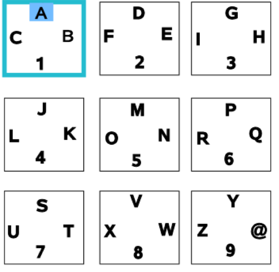
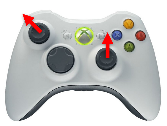
“While using the Xbox program ‘Xbox FTP Client’, I stumbled upon this alternative to the tried-and-true approach. The letters are placed like those on a phone pad, three letters and a number to each box. The left analog stick is used to select the box, and the right analog stick is used to highlight the letter/number of your choosing. Once the appropriate glyph is highlighted, you pull the right trigger with your index finger (a very natural motion, with both thumbs resting on the analog sticks) to select the letter/number. Once familiar with the interface, I’ve found I can type my name (‘ryan young’) in about 20 seconds, whereas it takes about 50 seconds with a traditional cursor and keyboard combination.” (example from Ryan Young)
Let’s think about this interface with respect to:
- learnability (direct or natural mapping? different kinds of consistency?)
- efficiency
Human Information Processing
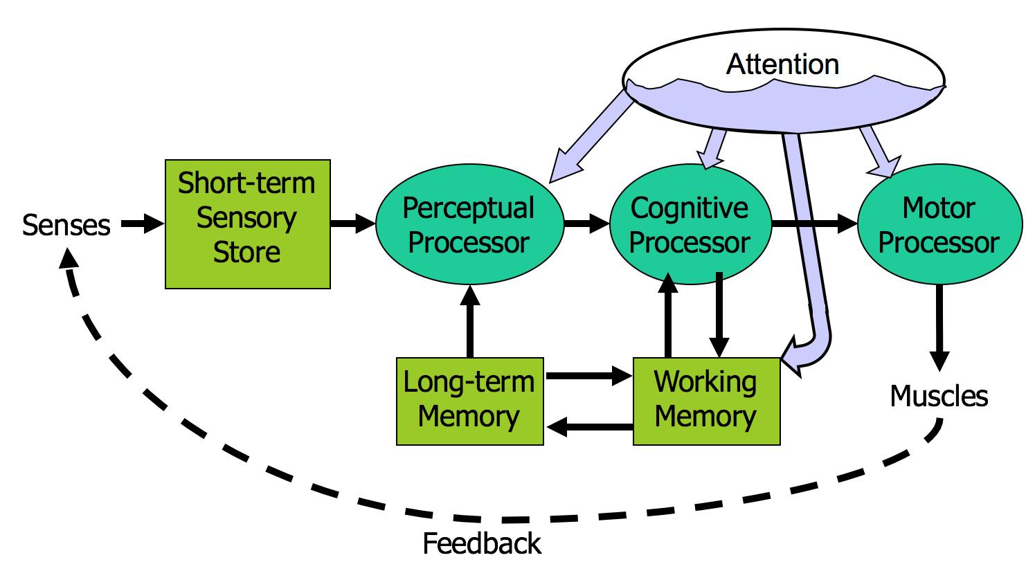
Here’s a high-level look at the cognitive abilities of a human being – really high level, like 30,000 feet. This is a version of the Model Human Processor (MHP), which was developed by Card, Moran, and Newell as a way to summarize decades of psychology research in an engineering model (Card, Moran, Newell, The Psychology of Human-Computer Interaction, Lawrence Erlbaum Associates, 1983).
This model is different from the original MHP; we’ve modified it to include a component representing the human’s attention resources (Wickens, Engineering Psychology and Human Performance, Charles E. Merrill Publishing Company, 1984).
This model is an abstraction, of course. But it’s an abstraction that actually gives us numerical parameters describing how we behave. Just as a computer has memory and processor, so does our model of a human. Actually, the model has several different kinds of memory, and several different processors.
Input from the eyes and ears is first stored in the short-term sensory store. As a computer hardware analogy, this memory is like a frame buffer, storing a single frame of perception.
The perceptual processor takes the stored sensory input and attempts to recognize symbols in it: letters, words, phonemes, icons. It is aided in this recognition by the long-term memory, which stores the symbols you know how to recognize.
The cognitive processor takes the symbols recognized by the perceptual processor and makes comparisons and decisions. It might also store and fetch symbols in working memory (which you might think of as RAM, although it’s pretty small). The cognitive processor does most of the work that we think of as “thinking”.
The motor processor receives an action from the cognitive processor and instructs the muscles to execute it. There’s an implicit feedback loop here: the effect of the action (either on the position of your body or on the state of the world) can be observed by your senses, and used to correct the motion in a continuous process.
Finally, there is a component corresponding to your attention, which might be thought of like a thread of control in a computer system. Note that this model isn’t meant to reflect the anatomy of your nervous system. There probably isn’t a single area in your brain corresponding to the perceptual processor, for example. But it’s a useful abstraction nevertheless.
- Processors have a cycle time
- T_p ~ 100ms [50-200 ms]
- T_c ~ 70ms [30-100 ms]
- T_m ~ 70ms [25-170 ms]
The main property of a processor is its cycle time, which is analogous to the cycle time of a computer processor. It’s the time needed to accept one input and produce one output.
Like all parameters in the MHP, the cycle times shown above are derived from a survey of psychological studies. Each parameter is specified with a typical value and a range of reported values. For example, the typical cycle time for perceptual processor, T_p, is 100 milliseconds, but various psychology studies over the past decades have reported mean cycle times between 50 and 200 milliseconds. The reason for the range is not only variance in individual humans; it is also varies with conditions. For example, the perceptual processor is faster (shorter cycle time) for more intense stimuli, and slower for weak stimuli. You can’t read as fast in the dark. Similarly, your cognitive processor actually works faster under load. Consider how fast your mind works when you’re driving or playing a video game, relative to sitting quietly and reading. The cognitive processor is also faster on practiced tasks.
It’s reasonable, when we’re making engineering decisions, to deal with this uncertainty by using all three numbers, not only the nominal value but also the range.
We’ve already encountered one interesting effect of the perceptual processor: perceptual fusion. Here’s an intuition for how fusion works. Every cycle, the perceptual processor grabs a frame (snaps a picture). Two events occurring less than the cycle time apart are likely to appear in the same frame. If the events are similar – e.g., Mickey Mouse appearing in one position, and then a short time later in another position – then the events tend to fuse into a single perceived event – a single Mickey Mouse, in motion.
Fusion also strongly affects our perception of causality. If one event is closely followed by another – e.g., pressing a key and seeing a change in the screen – and the interval separating the events is less than T_p, then we are more inclined to believe that the first event caused the second.
The cognitive processor is responsible for making comparisons and decisions. Cognition is a rich, complex process. The best-understood aspect of it is skill-based decision making. A skill is a procedure that has been learned thoroughly from practice; walking, talking, pointing, reading, driving, typing are skills most of us have learned well. Skill-based decisions are automatic responses that require little or no attention. Since skill-based decisions are very mechanical, they are easiest to describe in a mechanical model like the one we’re discussing.
Two other kinds of decision making are rule-based, in which the human is consciously processing a set of rules of the form if X, then do Y; and knowledge-based, which involves much higher-level thinking and problem-solving.
Rule-based decisions are typically made by novices or occasional performers of a task. When a student driver approaches an intersection, for example, they must think explicitly about what they need to do in response to each possible condition (“is there a stop sign? Are there other cars arriving at the intersection? Who has the right of way?”). With practice, the rules become skills, and you don’t think about how to do them anymore.
Knowledge-based decision making is used to handle unfamiliar or unexpected problems, such as figuring out why your car won’t start.
We’ll focus on skill-based decision making for the purposes of this reading, because it’s well understood, and because efficiency is most important for well-learned procedures.
- Open-loop control
- Motor processor runs a program by itself
- cycle time is T_m ~ 70 ms
- Closed-loop control
- Muscle movements (or their effect on the world) are perceived and compared with desired result
- cycle time is T_p + T_c + T_m ~ 240 ms
The motor processor can operate in two ways. It can run autonomously, repeatedly issuing the same instructions to the muscles. This is “open-loop” control; the motor processor receives no feedback from the perceptual system about whether its instructions are correct. With open loop control, the maximum rate of operation is one cycle every T_m ~ 70 ms.
The other way is “closed-loop” control, which has a complete feedback loop. The perceptual system looks at what the motor processor did, and the cognitive system makes a decision about how to correct the movement, and then the motor system issues a new instruction. At best, the feedback loop needs one cycle of each processor to run, or T_p + T_c + T_m ~ 240 ms.
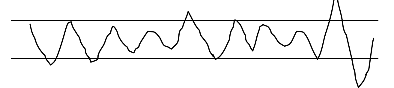
Here’s a simple but interesting experiment that you can try: take a sheet of lined paper and scribble a sawtooth wave back and forth between two lines, going as fast as you can but trying to hit the lines exactly on every peak and trough. Do it for 5 seconds. The frequency of the sawtooth carrier wave is dictated by open-loop control, so you can use it to derive your T_m. The frequency of the wave’s envelope, the corrections you had to make to get your scribble back to the lines, is closed-loop control. You can use that to derive your value of T_p + T_c.
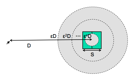
- Time T to move your hand to a target of size S at distance D away is:
T = RT + MT = a + b log (D/S + 1)
- Moving your hand to a target is closed-loop control
- Each cycle covers remaining distance D with error εD
Fitt’s Law
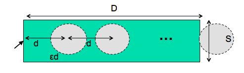
Steering Law
- Time T to move your hand through a tunnel of length D and width S is: T = a + b D/S
We already appealed to this model of closed-loop motor control to help explain why Fitts’s Law is logarithmic in distance and size, while the steering law is linear.
Simple reaction time – responding to a single stimulus with a single response – takes just one cycle of the human information processor, i.e. T_p+T_c+T_m.
But if the user must make a choice – choosing a different response for each stimulus – then the cognitive processor may have to do more work. The Hick-Hyman Law of Reaction Time shows that the number of cycles required by the cognitive processor is proportional to amount of information in the stimulus. For example, if there are N equally probable stimuli, each requiring a different response, then the cognitive processor needs log N cycles to decide which stimulus was actually seen and respond appropriately. So if you double the number of possible stimuli, a human’s reaction time only increases by a constant.
Keep in mind that this law applies only to skill-based decision making; we assume that the user has practiced responding to the stimuli, and formed an internal model of the expected probability of the stimuli.
- Accuracy varies with reaction time
- Here, accuracy is probability of slip or lapse
- Can choose any point on curve
- Can move curve with practice
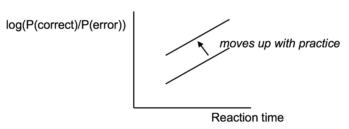
Another important phenomenon of the cognitive processor is the fact that we can tune its performance to various points on a speed-accuracy tradeoff curve. We can force ourselves to make decisions faster (shorter reaction time) at the cost of making some of those decisions wrong. Conversely, we can slow down, take a longer time for each decision and improve accuracy. It turns out that for skill-based decision making, reaction time varies linearly with the log of odds of correctness; i.e., a constant increase in reaction time can double the odds of a correct decision.
The speed-accuracy curve isn’t fixed; it can be moved up by practicing the task. Also, people have different curves for different tasks; a pro tennis player will have a high curve for tennis but a low one for surgery.
One consequence of this idea is that efficiency can be traded off against safety. Most users will seek a speed that keeps slips to a low level, but doesn’t completely eliminate them.
One more relevant feature of the entire perceptual-cognitive-motor system is that the time to do a task decreases with practice. In particular, the time decreases according to a power law. The power law describes a linear curve on a log-log scale of time and number of trials.
In practice, the power law means that novices get rapidly better at a task with practice, but then their performance levels off to nearly flat (although still slowly improving).
reading exercises
What is the most relevant model to consider when deciding how many items to put at the top level of a right-click menu?
(missing explanation)
Keystroke level model
Now we’re going to turn to the question of how we can predict the efficiency of a user interface before we build it. Predictive evaluation is one of the holy grails of usability engineering. There’s something worthy of envy in other branches of engineering–even in computer systems and computer algorithm design–in that they have techniques that can predict (to some degree of accuracy) the behavior of a system or algorithm before building it. Order-of-growth approximation in algorithms is one such technique. You can, by analysis, determine that one sorting algorithm takes O(n log n) time, while another takes O(n^2) time, and decide between the algorithms on that basis. Predictive evaluation in user interfaces follows the same idea.
At its heart, any predictive evaluation technique requires a model for how a user interacts with an interface. This model needs to be abstract – it can’t be as detailed as an actual human being (with billions of neurons, muscles, and sensory cells), because it wouldn’t be practical to use for prediction.
It also has to be quantitative, i.e., assigning numerical parameters to each component. Without parameters, we won’t be able to compute a prediction. We might still be able to do qualitative comparisons, such as we’ve already done to compare, say, Mac menu bars with Windows menu bars, or cascading submenus. But our goals for predictive evaluation are more ambitious.
These numerical parameters are necessarily approximate; first because the abstraction in the model aggregates over a rich variety of different conditions and tasks; and second because human beings exhibit large individual differences, sometimes up to a factor of 10 between the worst and the best. So the parameters we use will be averages, and we may want to take the variance of the parameters into account when we do calculations with the model.
Where do the parameters come from? They’re estimated from experiments with real users. The numbers seen here for the general model of human information processing (e.g., cycle times of processors and capacities of memories) were inferred from a long literature of cognitive psychology experiments. But for more specific models, parameters may actually be estimated by setting up new experiments designed to measure just that parameter of the model.
Predictive evaluation doesn’t need real users (once the parameters of the model have been estimated, that is). Not only that, but predictive evaluation doesn’t even need a prototype. Designs can be compared and evaluated without even producing design sketches or paper prototypes, let alone code.
Another key advantage is that the predictive evaluation not only identifies usability problems, but actually provides an explanation of them based on the theoretical model underlying the evaluation. So it’s much better at pointing to solutions to the problems than either inspection techniques or user testing. User testing might show that design A is 25% slower than design B at a doing a particular task, but it won’t explain why. Predictive evaluation breaks down the user’s behavior into little pieces, so that you can actually point at the part of the task that was slower, and see why it was slower.
The first predictive model was the keystroke level model (proposed by Card, Moran & Newell, “The Keystroke Level Model for User Performance Time with Interactive Systems”, CACM, v23 n7, July 1978).
This model seeks to predict efficiency (time taken by expert users doing routine tasks) by breaking down the user’s behavior into a sequence of the five primitive operators shown here.
Most of the operators are physical–the user is actually moving their muscles to perform them. The M operator is different–it’s purely mental (which is somewhat problematic, because it’s hard to observe and estimate). The M operator stands in for any mental operations that the user does. M operators separate the task into chunks, or steps, and represent the time needed for the user to recall the next step from long-term memory.
Here’s how to create a keystroke level model for a task.
First, you have to focus on a particular method for doing the task. Suppose the task is deleting a word in a text editor. Most text editors offer a variety of methods for doing this, e.g.:
- click and drag to select the word, then press the Del key
- click at the start and shift-click at the end to select the word, then press the Del key
- click at the start, then press the Del key N times
- double-click the word, then select the Edit/Delete menu command; etc.
Next, encode the method as a sequence of the physical operators: K for keystrokes, B for mouse button presses or releases, P for pointing tasks, H for moving the hand between mouse and keyboard, and D for drawing tasks.
Next, insert the mental preparation operators at the appropriate places, before each chunk in the task. Some heuristic rules have been proposed for finding these chunk boundaries.
Finally, using estimated times for each operator, add up all the times to get the total time to run the whole method.
The operator times can be estimated in various ways.
Keystroke time can be approximated by typing speed. Second, if we use only an average estimate for K, we’re ignoring the 10x individual differences in typing speed.
Button press time is approximately 100 milliseconds. Mouse buttons are faster than keystrokes because there are far fewer mouse buttons to choose from (reducing the user’s reaction time) and they’re right under the user’s fingers (eliminating lateral movement time), so mouse buttons should be faster to press. Note that a mouse click is a press and a release, so it costs 0.2 seconds in this model.
Pointing time can be modelled by Fitts’s Law, but now we’ll actually need numerical parameters for it. Empirically, you get a better fit to measurements if the index of difficulty is log(D/S+1); but even then, differences in pointing devices and methods of measurement have produced wide variations in the parameters (some of them seen here). There’s even a measurable difference between a relaxed hand (no mouse buttons pressed) and a tense hand (dragging). Also, using Fitts’s Law depends on keeping detailed track of the location of the mouse pointer in the model, and the positions of targets on the screen. An abstract model like the keystroke level model dispenses with these details and just assumes that T ~ 1.1s for all pointing tasks. If your design alternatives require more detailed modeling, however, you would want to use Fitts’s Law more carefully.
Drawing time, likewise, can be modeled by the steering law: T = a + b (D/S).
Homing time is estimated by a simple experiment in which the user moves their hand back and forth from the keyboard to the mouse.
Finally we have the Mental operator. The M operator does not represent planning, problem solving, or deep thinking. None of that is modeled by the keystroke level model. M merely represents the time to prepare mentally for the next step in the method–primarily to retrieve that step (the thing you’ll have to do) from long-term memory. A step is a chunk of the method, so the M operators divide the method into chunks.
The time for each M operator was estimated by modeling a variety of methods, measuring actual user time on those methods, and subtracting the time used for the physical operators–the result was the total mental time. This mental time was then divided by the number of chunks in the method. The resulting estimate (from the 1978 Card & Moran paper) was 1.35 sec–unfortunately large, larger than any single physical operator, so the number of M operators inserted in the model may have a significant effect on its overall time. (The standard deviation of M among individuals is estimated at 1.1 sec, so individual differences are sizeable too.) Kieras recommends using 1.2 sec based on more recent estimates.
One of the trickiest parts of keystroke-level modeling is figuring out where to insert the M’s, because it’s not always clear where the chunk boundaries are in the method. Here are some heuristic rules, suggested by Kieras (“Using the Keystroke-Level Model to Estimate Execution Times”, 2001).
Here are keystroke-level models for two methods that delete a word.
The first method clicks at the start of the word, shift-clicks at the end of the word to highlight it, and then presses the Del key on the keyboard. Notice the H operator for moving the hand from the mouse to the keyboard. That operator may not be necessary if the user uses the hand already on the keyboard (which pressed Shift) to reach over and press Del.
The second method clicks at the start of the word, then presses Del enough times to delete all the characters in the word.
Comparing designs & methods
Parametric analysis
Keystroke level models can be useful for comparing efficiency of different user interface designs, or of different methods using the same design.
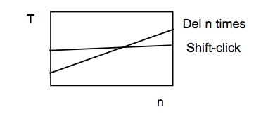
One kind of comparison enabled by the model is parametric analysis–e.g., as we vary the parameter n (the length of the word to be deleted), how do the times for each method vary?
Using the approximations in our keystroke level model, the shift-click method is roughly constant, while the Del-n-times method is linear in n. So there will be some point n below which the Del key is the faster method, and above which Shift-click is the faster method. Predictive evaluation not only tells us that this point exists, but also gives us an estimate for n.
But here the limitations of our approximate models become evident. The shift-click method isn’t really constant with n–as the word grows, the distance you have to move the mouse to click at the end of the word grows likewise. Our keystroke-level approximation hasn’t accounted for that, since it assumes that all P operators take constant time. On the other hand, Fitts’s Law says that the pointing time would grow at most logarithmically with n, while pressing Del n times clearly grows linearly. So the approximation may be fine in this case.
The developers of the KLM model tested it by comparing its predictions against the actual performance of users on 11 different interfaces: 3 text editors, 3 graphical editors, and 5 command-line interfaces like FTP and chat.
28 expert users were used in the test, most of whom used only one interface, the one they were expert in.
The tasks were diverse but simple: e.g. substituting one word with another; moving a sentence to the end of a paragraph; adding a rectangle to a diagram; sending a file to another computer. Users were told the precise method to use for each task, and given a chance to practice the method before doing the timed tasks.
Each task was done 10 times, and the observed times are means of those tasks over all users.
The results are in figure 6 of Card, Moran & Newell, “The Keystroke Level Model for User Performance Time with Interactive Systems“, CACM, v23 n7, July 1978.
The predicted time for most tasks is within 20% of the actual time. For perspective, civil engineers usually expect that their analytical models will be within 20% error in at least 95% of cases, so KLM is getting close to that.
One flaw in this study is the way they estimated the time for mental operators–it was estimated from the study data itself, rather than from separate, prior observations.
Keystroke level models have some limitations–we’ve already discussed the focus on expert users and efficiency. But KLM also assumes no errors made in the execution of the method, which isn’t true even for experts. Methods may differ not just in time to execute but also in propensity of errors, and KLM doesn’t account for that. KLM also assumes that all actions are serialized, even actions that involve different hands (like moving the mouse and pressing down the Shift key). Real experts don’t behave that way; they overlap operations.
KLM also doesn’t have a fine-grained model of mental operations. Planning, problem solving, different levels of working memory load can all affect time and error rate; KLM lumps them into the M operator.
reading exercises
Which of the following user interface tasks might be usefully modeled by KLM?
(missing explanation)
GOMS
GOMS is a richer model that considers the planning and problem solving steps. Starting with the low-level Operators and Methods provided by KLM, GOMS adds on a hierarchy of high-level Goals and subgoals (like we looked at for task analysis) and Selection rules that determine how the user decides which method will be used to satisfy a goal.
Here’s an outline of a GOMS model for the text-deletion example we’ve been using. Notice the selection rule that chooses between two methods for achieving the goal, based on an observation of how many characters need to be deleted.
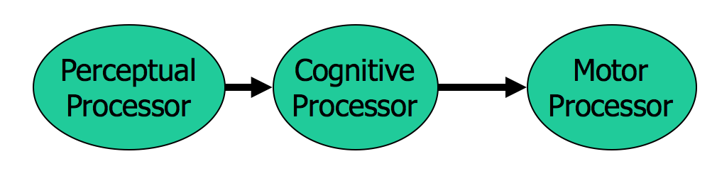
- CPM-GOMS models parallel operations
- e.g. point & shift-click
- Uses parallel cognitive model
- each processor is serial
- different processors run in parallel
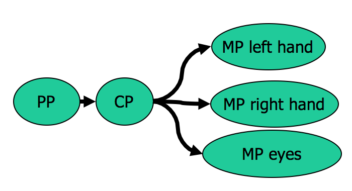
CPM-GOMS (Cognitive-Motor-Perceptual) is another variant of GOMS, which is even more detailed than the keystroke-level model. It tackles the serial assumption of KLM, allowing multiple operators to run at the same time. The parallelism is dictated by a model very similar to the Card/Newell/Moran information processing model we saw earlier. We have a perceptual processor (PP), a cognitive processor (CP), and multiple motor processors (MP), one for each major muscle system that can act independently. For GUI interfaces, the muscles we mainly care about are the two hands and the eyes. The model makes the simple assumption that each processor runs tasks serially (one at a time), but different processors run in parallel.
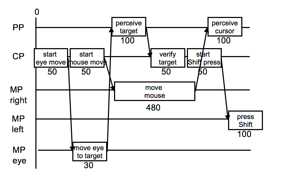
We build a CPM-GOMS model as a graph of tasks. Here’s the start of a Point-Shift-click operation.
First, the cognitive processor (which initiates everything) decides to move your eyes to the pointing target, so that you’ll be able to tell when the mouse pointer reaches it.
Next, the eyes actually move (MP eye), but in parallel with that, the cognitive processor is deciding to move the mouse. The right hand’s motor processor handles this, in time determined by Fitts’s Law. While the hand is moving, the perceptual processor and cognitive processor are perceiving and deciding that the eyes have found the target. Then the cognitive processor decides to press the Shift key, and passes this instruction on to the left hand’s motor processor.
In CPM-GOMS, what matters is the critical path through this graph of overlapping tasks – the path that takes the longest time, since it will determine the total time for the method.
Notice how much more detailed this model is! This would be just P K in the KLM model. With greater accuracy comes a lot more work.
Another issue with CPM-GOMS is that it models extreme expert performance, where the user is working at or near the limits of human information processing speed, parallelizing as much as possible, and yet making no errors.
How can we think about today’s Hall of Fame and Shame example, the XBox FTP Client keyboard, in light of the CPM-GOMS model?
CPM-GOMS had a real-world success story. NYNEX (a phone company) was considering replacing the workstations of its telephone operators. The redesigned workstation they were thinking about buying had different software and a different keyboard layout. It reduced the number of keystrokes needed to handle a typical call, and the keyboard was carefully designed to reduce travel time between keys for frequent key sequences. It even had four times the bandwidth of the old workstation (1200 bps instead of 300). A back-of-the-envelope calculation, essentially using the KLM model, suggested that it should be 20% faster to handle a call using the redesigned workstation. Considering NYNEX’s high call volume, this translated into real money – every second saved on a 30-second operator call would reduce NYNEX’s labor costs by $3 million/year.
But when NYNEX did a field trial of the new workstation (an expensive procedure which required retraining some operators, deploying the workstation, and using the new workstation to field calls), they found it was actually 4% slower than the old one.
A CPM-GOMS model explained why. Every operator call started with some “slack time”, when the operator greeted the caller (e.g. “Thank you for calling NYNEX, how can I help you?”) Expert operators were using this slack time to set up for the call, pressing keys and hovering over others. So even though the new design removed keystrokes from the call, the removed keystrokes occurred during the slack time – not on the critical path of the call, after the greeting. And the 4% slowdown was due to moving a keystroke out of the slack time and putting it later in the call, adding to the critical path. On the basis of this analysis, NYNEX decided not to buy the new workstation. (Gray, John, & Atwood, “Project Ernestine: Validating a GOMS Analysis for Predicting and Explaining Real-World Task Performance”, Human-Computer Interaction, v8 n3, 1993).
This example shows how predictive evaluation can explain usability problems, rather than merely identifying them (as the field study did).