The goal of this research project is to develop a Three-Dimensional Holographic Imaging system for aquatic species. The 3D Holographic camera will be carried inside an Underwater Autonomous Vehicle (UAV) that will be sent in an exploration mission to a depth of around 11,000 meters, currently the greatest depth attempted to image aquatic ecosystems. Figure 1 shows a sketch of a possible deployment.

Figure 1

The images are recorded in a high-resolution CCD sensor using Digital Holography in a lens-free in-line configuration. The captured images (holograms) contain information about the phase and amplitude of the optical field propagated after illuminating the desired object. This information is encoded in the hologram as a set of fringes that are later decoded using image-processing algorithms to recover the intensity distribution at an image plane. This is located at a distance similar to the distance from the object to the CCD camera. Figure 2 shows the typical in-line setup.

Figure 2

In most of the experiments a plane-wave is used as a reference interfering with the field scattered by the object at the detector plane. The recorded intensity is then:

(1)

Where:

: is the reference wave
: is the object wave

If we expand equation (1) we get:

(2)

In equation (2) the first two terms represent the so-called “DC term”, while the third and fourth term are the real and virtual images respectively. In order to recover the real image the first step is to multiply equation (2) by a digital replica of the conjugate of the reference wave. In this step we are assuming that the effect of the DC term is weak so it can be neglected.

(3)

The virtual image is out-of-focus and, as shown in the experiments below, its effect for small objects at large distances is very small. For this reason it can also be neglected.

The second step in the reconstruction algorithm is to apply a Fresnel transformation given by:

(4)

After paraxial approximations:

Where:

: is the reconstructed field at the image plane
is the wavelength used to record the hologram
is the transformation kernel and is given by:

The rest of the coordinates are shown in figure 3:

Figure 3

The paraxial approximated transformation kernel has an analytic Fourier transform given by:

This allows us to implement the “convolution approach” for the reconstruction. In the convolution approach all the computations are made in the Fourier domain using the fast-Fourier-transform algorithms to make the reconstruction faster. Figure 4 shows the block diagram followed for the case of in-line configuration with a plane reference wave.

Figure 4

The dependence in distance of H allows us to “digitally scan” in the longitudinal direction. In other words, we can reconstruct the fields at different planes. In the case of two objects located at different distances from the CCD camera, if we set the reconstruction distance equal to the distance from the first object to the detector plane, the second object will appear blurry while the first one will be in focus. Therefore, the 3D coordinates of an object can also be retrieved. The scanning process is exemplified in the following animation:

Click on the image to run animation

Figure 5 shows the optical set-up for an experiment in the laboratory. The first target objects were brine shrimp swimming freely in a tank filled with seawater. Digital Holograms were created using a He-Ne laser (632.8nm) and a CCD camera KAF-16801E from Kodak. The CCD camera is a full-frame sensor with 4096x4096 pixels and a pixel size of 9 microns. A mechanical shutter controlled by a monostable multivibrator circuit synchronized with the CCD camera was used to set the integration time to 2ms.

Figure 5

Figure 6 shows a typical hologram recorded using an in-line configuration with a plane reference-wave.

Figure 6

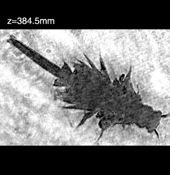
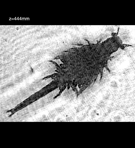
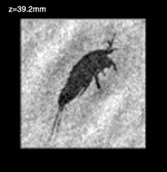
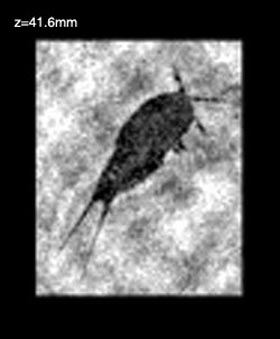
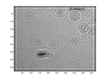
The following are some reconstructions of brine shrimp captured at short, medium and large distances from the CCD camera. The sampled brine shrimp ranged between 2-5mm in length.

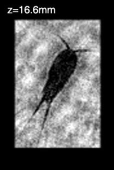
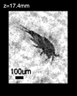
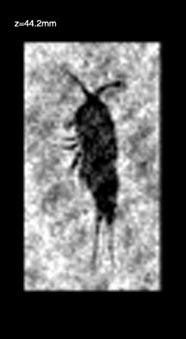
In the next set of experiments copepods swimming freely in a tank were imaged. The length of the imaged copepods ranged between 100-400 m m. The following images are some reconstruction made for different distances from the CCD camera.

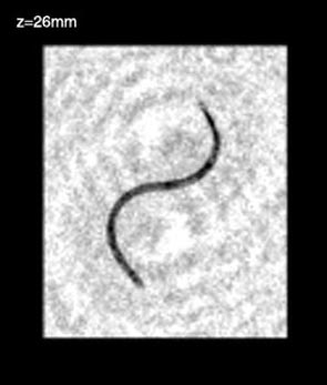
Similarly, the following are some reconstructions of live aquatic species found in the sample of seawater imaged:

As explained above, we digitally scan for several reconstruction distances from a single hologram. An example of this procedure is shown in the movie below:

Click on the image to run the movie

We are currently working in reducing the size of the imaging system. In addition, a pulsed laser will be implemented to reduce the motion of the UAV to less than one pixel.

Other configurations are also being explored, such as: off-axis, reflective (backward-scattering), spherical reference-wave, high-pass Fourier-filter, Mach-Zehnder among others.

ADDITIONAL LINKS:

Autonomous Multi-Scale Digital Imaging of Ocean Species

Digital Holographic Imaging of Microstructured and Biological Objects

BACK TO TOP