Due: Part I is due Tuesday, March 13, 2018, at 4:00 pm on Stellar
Part II is only required for
11.521 and due Tuesday, April 3, 2018, at 4:00 pm (the class after Spring
Break)
A housing value 'surface' for Boston would show the high and low value neighborhoods much like an elevation map shows height. The computation needed to do such interpolations involve lots of proximity-dependent calculations that are much easier using a so-called 'raster' data model instead of the vector model that we have been using. Thus far, we have represented spatial featuressuch as Boston parcel or block group polygonsby the sequence of boundary points that need to be connected to enclose the border of each spatial objectfor example, a parcel, a city block, or a Census block group. A raster model would overlay a grid (of fixed cell size) over all of Boston and then assign a numeric value (such as the block group ID or median housing value) to each grid cell depending upon, say, which block group or parcel contained the center of the grid cell. Depending upon the grid cell size that is chosen, such a raster model can be convenient but coarse-grained with jagged boundaries, or fine-grained but overwhelming in the number of cells that must be encoded.
In this exercise, we only have time for a few of the many types of spatial analyses and spatial smoothing algorithms that are possible using raterized datasets. Remember that our immediate goal is to use the Boston sales data to generate a housing-value 'surface' for Boston. (Actually, to keep the computations manageable for a short exercise, we'll compute the surface only for East Boston.) We'll do this by 'rasterizing' the sales data and then recomputing the value of each grid cell based not only on the housing value of any sales that fall within each grid cell but also on the value of nearby homes that sold. As usual, accomplishing this by mixing and matching the specific data and tools that we have in Postgres, ArcGIS, and MS-Access is somewhat more complex and frustrating than we might expect. The point of the lab exercise is not to 'memorize' all the tricks and traps involved, but to understand the complexities and ways around them so that you can 'reverse engineer' a new problem that might be doable if decomposed into particular, doable data processing, model building, and visualization steps.
Here is a link to the topic outline and notes for today's in-class lab presentation: lab5_inclass.txt
Copy the familiar ./data/eboston05 folder from the class data locker into a local folder such as C:\temp\lab5. In addition, unzip a new file .data/boston96.zip into the same local folder C:\temp\lab5. You should end up with a two folders named 'eboston05' and 'boston96' in your local C:\temp\lab5 folder. This boston96 folder contains all the new shapefiles we need for this exercise plus a personal geodatabase (11.521_boston96_gdb.mdb) that has MS-Access versions of the Postgres tables that we will use. The boston96 folder also contains an ArcMap document, boston96_lab5start.mxd, that gets you started with the familiar shapefiles from 'eboston05' plus the new ones that we will use today. The ArcMap document was saved using relative address so, if you opened it from inside of C:\temp\lab5\boston96 and the eboston05 folder is also in C:\temp\lab5 then ArcMap should be able to find the location of all the needed shapefiles.
/***** Alternative ArcMap startup steps *********/
Instead of starting with boston06_lab5start.mxd, we could open the familiar eboston05_lab2start.mxd document and add the new shapefiles since they are included elsewhere in our data locker. Use ArcCatalog to copy the additional shapefiles listed below from the class data locker into your local folder (C:\TEMP\LAB5).
Next, open ArcMap by double-clicking on your local copy of eboston05_lab2start.mxd in the c:\temp\lab5\eboston05 folder. Add to ArcMap your local copy of the additional shapefiles listed above and then prune the shapefile list and rearrange their order as listedbelow: (Just check to be sure that your Data Frame is set to Mass State Plane (mainland) NAD83 meters coordinates. Note, also, that we include a second 1996 shapefile for East Boston parcels instead of just the ebos_parcels05 version that we have already used.)
/****** end of alternative ArcMap startup steps ******/
If necessary, rearrange the ordering of layers in ArcMap as follows:
To get started with a useful visualization of Boston, we suggest the
following setup: Adjust (if necessary) the colors and transparency
of the layers so that the ocean is blue with no border, and the Planning
District boundaries for Boston are visible and other shapefiles are turned
off.
MAP #1: Create a thematic map of median housing value by shading the boston_bg90 block group theme of 1990 census data based on the 1990 medhhval values. Be sure to exclude block groups with medhhval = 0 and use the default 'natural breaks' classification. Since many block groups had too small a sample of housing that is owned rather than rented, many block groups get excluded from your thematic map.
To reduce clutter and avoid coordinate system conflicts let's add a new
Data Frame that we will use for our raster operations. Click on Insert/Data_Frame
and rename the new data frame 'East Boston Raster'. In
the next section, we will divide East Boston into 50 meter grid
cells. The boundary of East Boston that is included in bos_planning_districts
will be the most convenient shapefile that we have to provide a
bounding box for East Boston. However, that shapefile is saved on disk in
NAD83 Mass State Plane coordinates (feet) rather than in NAD83 Mass State
Plane coordinates (meters). Beware of the coordinate system of your Data
Frame and your data layers: If you started your ArcMap session using eboston05_lab2start.mxd
or boston96_lab5start.mxd, then the data frame will be
set to Mass State Plane (NAD83-meters). However, if you started with a
blank ArcMap session and then first added the East Boston parcels (or
planning districts), then the coordinate system of the parcel shapefile
(which is Mass State Plane NAD83-feet) will be adopted by
the data frame. Then, when you set a grid cell size of '50' the units will
be 50 feet not 50 meters. We suggest that you use the
bos_planning_districts shapefile for the 'mask' that isolates the East
Boston area for your raster grid. But this shapefile is saved on disk in
Mass State Plane NAD83-feet. Convert it to Mass State Plane NAD83-meters
on disk and use that layer to build your East Boston 50x50m grid cells.
When you do spatial operations (like converting vector to raster or
spatial joins) you will find ArcGIS to be more reliable if each data layer
is saved on disk in the same coordinate system. To save a new copy of
bos_planning_districts in NAD83 Mass State Plane (meters), right click on
the layer, choose Data/Export-data and then be sure to use the same
coordinate system as 'the data frame'. For the storage
location, browse to C:\temp\lab5, name it bos_districts_meters and
save as file type: shapefile. (If you are familiar with
geodatabases, you can save it there but you might have a harder time
finding it again later on.) Allow this new shapefile to be added to
your ArcMap session and then copy and paste it into your new 'East Boston
Raster' data frame. Then, copy and paste the 'ESRI_World_Shaded_Relief'
and 'Mass Data from MassGIS GeoServer' layers into the new data frame (for
visualization purposes) and you are ready to construct your 50 meter grid
cells and begin the raster analysis.
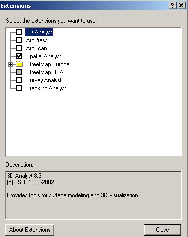
ArcGIS's raster manipulation tools are bundled with its Spatial Analyst extension. This section reviews how to setup Spatial Analyst in case you have forgotten how or you learned about raster analysis using another GIS package. While ArcGIS 10 has all the raster functionality of earlier versions, many of the menus have changed. Indeed, this exercise was first written with earlier versions and we may have overlooked some of the changes in how you access the raster tools! It's a big bundle so lets open ArcGIS's help system first to find out more about the tools. Open the ArcGIS help page from within ArcMap by clicking Help > ArcGIS Desktop help from the menu bar. I miss the 'index' that ArcGIS help used to have - the new search tool brings up too many subtopics. In our case, the easiest way to find out about 'spatial analyst' raster tools is to locate it under the 'extension' portion of the 'Contents / Extensions / Spatial Analyst tab. If you have not used spatial analyst for a while, be sure to browse through the overview section and check out the 'related topics.'. During the exercise, you'll find these online help pages helpful in clarifying the choices and reasoning behind a number of the steps that we will explore.
The Spatial Analyst module is an extension, so it must be loaded into ArcGIS separately. Prior to ArcMap version 10, 'Spatial Analyst' functions were accessed from a 'spatial analyst' toolbar that could be added to ArcMap once you turned on the Spatial Analyst extension. Beginning with version 10, ArcMap wants you to access spatial analyst functions via ArcToolbox. This is a more generic approach that facilitates the construction of data processing pipelines (as we shall see later with Model Builder). The Spatial Analyst toolbar is still available, however we do not recommend that you use it. Not only does it have small differences in parameter choices from the ArcToolbox operations, but the toolbar environment settings can differ from the ArcToolbox environment settings and that can lead to confusion. [Note the menu listed in the Fig. 1 graphic may differ slightly depending upon the machine and user account setup. Also, ArcGIS version 9 used 'Toolbar' menu instead of 'Customize' to load extensions.]
|
Although you just activated the "Spatial Analyst" extension, nothing changes in the ArcMap windows. You must open up ArcToolbox and navigate to the Spatial Analyst section (or add the Spatial Analyst tool bar) to see what specific tools are available. We want you to use ArcToolbox for these exercises so you will not have any use for the spatial analyst toolbar. [Nevertheless, if you want to activate the toolbar, right-click in the area of the toolbar space near the top of the ArcMap window to get the list of available toolbars. If you check the "Spatial Analyst" tool bar, it will become visible - but you will not need it.]
Choose 'ArcToolbox' from the Geoprocessing menu. (Alternatively, you could click the ArcToolbox icon in the 'standard' tool bar.) The ArcToolbox window pops up outside the ArcMap window. If you double-click the top of the window, it will jump inside of ArcMap! [NOTE: If you are familiar with the Spatial Analyst toolbar in the older ArcGIS versions, beware that some of the spatial analyst functions in ArcToolbox behave a little differently from the menu items in the 'spatial analyst' toolbar. In particular, ArcToolbox and the spatial analyst toolbar uses separate environment variables.]
If you have limited experience with raster-based GIS analysis, review the ArcGIS online help as well as the notes and exercises on raster analysis from the Fall 11.520 class. In particular, see this lab exercise: http://mit.edu/11.520/www/labs/lab7/lab7.html
NOTES:
Setting Analysis Properties:
Before building and using raster datasets, we should set the grid cell
sizes, the spatial extent of our grid, and the 'no data' regions that
we wish to 'mask' off. Let's begin by specifying a grid cell size of
50 meters and an analysis extent covering all of East Boston .[Remember,
we want you to do the exercise using only the ArcToolbox tools. The
environment settings for ArrcToolbox tools are available for editing via
'Geoprocessing / Environment' Expand the 'processing extent' and 'raster
analysis' section.]
To do this, click 'Spatial Analyst > Option '. When the "Options" window pops up.
If successful, the ebosgd layer will be added to the data frame window. Turn it on and notice that the shading covers all the grid cells whose center point falls inside of the spatial extent of the ebosgd layer. Note that the attribute table for ebosgd contains only one row and indicates that 5240 grid cells have the same value of 'East Boston' for the attribute field called NAME. (Attribute tables for raster layers contain one row for each unique grid cell value - hence, there is only one row in this case. Our 50 meter grid cells generate 112 rows and 98 columns for the bounding box that includes East Boston. (The Source tab in the ebosgd layer properties window lists the number of rows and columns in the raster. Note that 112 x 98 = 10,976 grid cells if your East Boston planning district layer had only East Boston in it. For all of Boston, there are 337x377= 127,049 cells. Restricting the grid cells further to those whose centroid falls within the East Boston boundary reduces the count to 5,240 cells. Note that if you use a slightly altered East Boston shapefile from another source, then the number of cells could be a bit higher or lower than 5,240.)
By this point, you should have created a new grid cell layer called ebosgd that has 50 meter grid cells [not 50 feet which you will get if you use Mass State Plane NAD83 FEET coordinate system that is associated with the Boston planning district shapefile].
A city assessor's database of all properties in the city would generally be considered a good estimate of housing values because the data set is complete and maintained by an agency which has strong motivation to keep it accurate. This database does have drawbacks, though. It is updated sporadically, people lobby for the lowest assessment possible for their property, and it's values often lag behind market values by many years.
Recent sales are another way to get at the question. On the one hand, their numbers are believable because the price results from an informed negotiation between a buyer and a seller that results in the 'true' value of the property being revealed (if you are a believer in the economic market-clearing model). However, some sales may not be 'arms length' (i.e., not representative of market value because they are foreclosure sales, sales to family members, etc.). In addition, the accuracy of such data sets are susceptible to short-lived boom or bust trends and, since individual houses (and lots) might be bigger or smaller than those typical of their neighborhood, individual sale prices may or may not be representative of housing prices in their neighborhood.
Alternatively, the census presents us with yet another opportunity for estimating housing valuethe median housing values aggregated to the block group level. However, this data set is also vulnerable to criticism from many angles. The numbers are self-reported, only a sample of the population is asked to report, and the data are aggregated up to the block group level. The benefit of census data is that they are cheaply available and they cover the entire country.
3.1 Pulling East Boston Data from the BOSTON.SALES Table
IMPORTANT NOTE: In this section, you will be creating views and importing data into ArcGIS. PLEASE, name all your views and tables adding your initials at the beginning, followed by an underscore i.e. jmg_holdsales1 (just so that everyone can create their own tables)
To begin exploring some of these ideas, we will use an Postgres table called sales containing information about the sale price of residential Boston parcels that sold between 1986 and 1995. (This sales tables and all the others that we use today are duplicated in the personal geodatabase boston96_lab5_gdb.mdb file included in boston96.zip and usable by MS-Access.) In Postgres, this sales table is stored under the boston96 schema (instead of public) of the class521 database. Make sure you specify the Schema search path to look first in boston96 for the table. One way is to run: set search_path to boston96,public; (Otherwise, you will need to prefix the table name with the schema name as in: boston96.sales) From PgAdmin or phpPgAdmin take a look at the sales table:
select *
from sales
order by sale_id asc
limit 30;

The first two characters of the parcel_id are the Ward number. Let's
see how many East Boston (Ward 01) sales are included in the BOSTON96.SALES
table: (Beware that this query works in Postgres but MS-Access does not
support the count(distinct fieldname) syntax within standard SQL).
select count(*), count(distinct parcel_id) as count_pid, count(distinct base_id)as count_bid
from sales
where substr(parcel_id, 1, 2) = '01';

Hmm, there are 2836 sales involving 1836 distinct parcel numbers and 1354
unique base_id values. Condos within the same building/development
share the same base_id (and parcel footprint) but have different
parcel numbers (the last 3 digits differ). Unfortunately, split parcels
can also retain the same base_idbut they have different
footprints as well as differing last three digits. For the purposes of
this exercise, we will ignore complications involving split parcels but
will address complications associated with condo sales and multiple sales
of individual parcels.
To begin, let's use the substring function (subsstr) to construct a SQL
query that lets us pull into ArcGIS the IDs and (average) sale price of all
Ward 01 parcels: create view public.jf_holdsales1 as select base_id, avg(cast(price as numeric)) as saleprice, count(*) as sales from boston96.sales where substr(base_id,1,2) = '01' group by base_id;
Make sure you prefix the view with the 'public.' schema name since you
are not allowed to create views within the 'boston96' schema. If
your search path looks first in 'boston96' and then in 'public' you can
say 'sales' rather than 'boston96.sales'.
There are 1354 rows in this tableincluding one base_id that showed up 84 times in the SALES table! (It is a condominium complex.) Let's look at the year in which each sale occurred. We can see this using the date manipulation function, to_char:
select to_char(saledate,'YYYY') as year, count(*)
from sales
where substr(parcel_id,1,2) = '01'
group by to_char(saledate,'YYYY')
order by to_char(saledate,'YYYY');
Hmm, most sales are indeed during the 10-year period 1986 through 1995 but there are a few earlier sales that we should probably omit from our analyses. Refine your view and save it as a table (call it <your initials>_ holdsales2) to include only those East Boston sales that occurred during 1986-1995. Download it as a .csv file and save it in a local directory, and pull it into ArcGIS using the techniques explained in Lab 4.
Summary of relevant Postgres tables for use in this lab:
These SQL queries can help us understand which columns are plausible primary keys:
select count(*), count(distinct parcel_id), count(distinct base_id)
  from boston96.parcel96;
-- 138001;138001;92161 --> parcel_id is assessing record, base_id is ground parcel ID
select count(*), count(distinct parcel96_), count(distinct parcel96_i), count(distinct parcel_id),
        count(distinct parcel_i_1), count(distinct base_id)
  from boston96.parcel96shp;
-- 101213;101213;6572;6551;99859;91982 --> parcel_i_1 should be a unique parcel/unit id and base_id a unique
ground parcel for joining to the assessing data.  However, there are some duplicates and we have used
parcel96_ as a primary key for the table.
3.2 Mapping East Boston Parcel Sales
There are about 100,000 ground parcels in Boston but, for this exercise, we will focus only on the 6500+ East Boston parcels that we have used in earlier labs. At this point, be sure that you have added the ebos_parcels05.shp shapefile to your ArcMap view. Note that the attribute table contains both a parcel_id and a base_id column. We could use base_id to join the holdsales2 table to 'ebos_parcels05.shp' and then do a thematic map based on sales price. (Try it later if you have time.) But many of the parcels are so small and the number of sales so many that the resulting thematic map of housing prices won't be too readable. In addition, the unsold parcels won't be shaded at all and parcels with multiple sales will only be shaded based on the value of the last sale.
Instead, we would like to construct an appropriate average of resales and nearby sales as an indication of housing value in the area surrounding the sale. One way to do such an interpolation is to compute a housing value for any particular location that is the average of, say, the nearest dozen sales. When computing the average, we might want to weight distant sales lower than close-by sales. By rasterizing the space within East Boston we can identify a finite and manageable number of places to consider (each grid cell) and then we can use the capacity of the GIS to know which sales are 'nearby.' (We don't have to rasterize East Boston. We could consider every parcel and set it's value to be a weighted average of its salesif anyand its neighbors. But that requires a lot more geometry calculations - e.g., to compute an adjancency matrix - so analysts often settle for a quicker raster analysis as illustrated next.) Let us handle the condo and multiple sale issue on the Postgres side and the neighborhood average smoothing on the ArcMap side.
It seems like we are 'almost there' but we will see shortly that there are several steps left. For example, some houses sold more than once, condos have multiple housing units on a single parcel, the 2005 parcel map uses different parcel IDs from the 1995 parcel map! Let us create a new view called xxx_holdsales3 that averages the sales price of all sales associated with a single ground parcel (base_id) during the 10 year period. A little inspection of eboston96.sales suggests that this may not be as simple as we would hope and we need several steps. Many 'base_id' fields are blank or incomplete and the 'condotag' column seems to either contain 'N' for non-condo or be blank. Also, we are not yet certain that the parcel_id in the sales table (for sales from 1985 through 1995) will match pid_long or base_id in the fiscal year 2005 assessing table for Boston. Let's do some checking on the Postgres side. The sales data are in boston96.sales, the attribute table from ebos_parcel05.shp is in an Postgres table called public.ebos_parcels05, and the FY05 assessing data is in public.bos05eb. Notice that we are working under the eboston database, but in multiple schemas, so we have to identify what schema our tables are located in and/or set the Schema path in our SQL query window.
Run a few SQL queries such as the following to get a sense of how well the files match up.
select count(*)
from boston96.sales s, bos05eb b
where substr(b.pid,1,2) = '01'
and s.parcel_id = b.pid
and cm_ID is not null;
	-- 892 rows


select count(*)
from boston96.sales s
where substr(s.parcel_id,1,2) = '01';
	-- 2836 rows


select count(*)
from bos05eb b
where substr(b.pid,1,2) = '01';
	-- 7235 rows
Groan! Only 892 of the 2836 parcel IDs in the sales table match any of the FY2005 parcel numbers. Something is wrong! Fortunately, we have saved a 1996 parcel map for Boston. That year is just at the end of the sales period for which we have data and happens to be before Boston did a renumbering of its parcels! The 1996 parcel shapefile is saved as parcel1996.shp (in NAD83 meters) in the class data locker K:\data\parcel1996.shp and the assessing data for 1996 in a form equivalent to the schema of bos05eb is saved in Postgres as a table called boston96.parcel96. For your convenience we have saved key attribute fields from for all 1996 Boston ground parcels with non-zero parcel_id into an Postgres table called boston96.parcel96shp. We have also saved the East Boston portion of parcel1996.shp into a smaller shapefile called ebos_parcels96.shp. This shapefile has also been added to the eboston05 subfolder of the class data locker: K:\data\eboston05 and should already be in the copy of that folder that you added to C:\TEMP.
Let us check how well the data from these 1996 files match up with the sales data.
select count(*)
from boston96.sales s, parcel96 b
where substr(b.parcel_id,1,2) = '01'
and s.parcel_id = b.parcel_id;
	-- 2737 rows
All but 99 East Boston sales records match. However, this match is for the assessing records - not the shapefile containing the ground parcels. Let us see if the field that looks like a complete ground parcel ID in the attribute table of ebos_parcels96.shp matches parcel_id in assess_data.sales:
select count(*)
from boston96.sales s, parcel96shp p
where substr(p.parcel_i_1,1,2) = '01'
and substr(p.parcel_i_1,1,7) = substr(s.parcel_id,1,7);
	-- 3109 rows - TOO MANY
Since condos have multiple records in both the sales table and the shapefile, we have extra matches. (Do you see why?) Let's try this query instead:
select count(*)
from (select distinct substr(parcel_id,1,7) as parcelsale
        from boston96.sales) s,
     (select distinct substr(parcel_i_1,1,7) as parcelshp
        from boston96.parcel96shp
       where substr(parcel_i_1,1,2) = '01') p
where p.parcelshp = s.parcelsale;
	-- 1347 rows
Hmm, now the number looks low! But maybe not: select count(distinct substr(parcel_id,1,7)) from sales where substr(parcel_id,1,2) = '01'; -- 1354 rows
Finally!! We see that there are 1354 unique East Boston ground parcels involved in residential sales during the 10 year period and all but 7 of the parcel IDs matched IDs in the shapefile. That looks pretty good.
Let's remind ourselves where we are at this point. We have two shapefiles of East Boston parcels from 2005 and from 1996: ebos_parcels05.shp and ebos_parcels96.shp. We also have the three Postgres tables boston96.sales, boston96.parcel96, and boston96..parcel96shp containing, for all of Boston, the 1985-1995 residential sales information, the 1996 assessing office information, and selected attributes from the ebos_parcels96.shp. Shortly, we will join the three Postgres tables together to pull off average sales prices for East Boston residential parcels and associate the prices with parcel IDs that can be located and mapped using the 1996 parcel shapefile. Whew! We then want to use these sales prices to interpolate a land value 'surface' for all the residential parts of East Boston, not just the ones that sold during our 10-year period.
We could use ebos_parcels96.shp for this purpose but it will be easier to do the interpolation if we join the sales data to a 'point' coverage rather than to a polygon coverage. (ArcGIS can 'rasterize' the parcel layer but doesn't have a simple interpolation option that will first compute a new price for each parcel polygon that is a (weighted) average of nearby parcels that have sold. But ArcGIS does have an interpolation option that will do such a nearest neighbor weighted average computation for a point layer.) Since we'll only have time today to show one of the simpler interpolation methods, we'll do that. You can create a point (centroid) shapefile for East Boston parcels by adding X and Y fields to your copy of the ebos_parcels96 attribute table and then using the Field/calculate-geometry choice from the attribute table options menu. However, there are a few 'gotchas' to consider before trying to do these calculations. First, it is more reliable to add fields to an attribute table when the table is not already joined (or related) to another table and you may have already joined the shapefile to the East Boston assessing table (parcel96). Second, the data frame is set to Mass State Plane NAD83 (in meters) but we have not yet checked the on-disk coordinate system for ebos_parcels96 (and it is NAD83 feet!). The fine print in ArcGIS help warns us that centroid calculations using 'calculate geometry' can only be done on layers that are being displayed in their native coordinate system.
If you want to be sure to avoid these two difficulties, add a fresh local copy of ebos_parcels96.shp into a new data frame with no other layers. Let us rename this to ebos_parcels96_xy.shp since we will change it by adding X/Y fields and we want to remember that it will be different from the original. Check that the data frame is in Mass State Plane meter coordinates - it should be since that is the coordinate system used by ebos_parcels96.shp on disk. (We could also calculate centroids using NAD83-feet if that were the coordinate system we used for the on-disk version of the shapefile). Now we can compute X/Y values for the parcel centroids in the native coordinates. Add two fields called CentX and CentY to the ebos_parcels96_xy attribute table and set the data type to double with precision=12 and scale=3. Now, right click each attribute column and use the 'calculate geometry' option to compute the X/Y centroid values.
Next, we want to create a point shapefile using the centroids. (Thus far, we have only added the centroid columns to the table but ebos_parcels96_xy.shp is still a shapefile of polygons.) Edit the properties of ebos_parcels96_xy.shp so that only the fields parcel_i_1 (which corresponds to pid_long in later years), wpb, CentX, and CentY are visible and open this attribute table. (It is okay to keep all the fields but these are the only ones that we really need.) Export these columns into a new DBF table on a writeable local drive with the name ebos_xydata.dbf. Finally, add this table to ArcMap and use the Display-XY-Data option (that we used in an earlier lab) to convert it to a new shapefile that the system will call 'ebos_xydata events'. When creating this shapefile of points, you may want to edit the coordinate system to state that it is Mass State Plane (mainland) NAD83 (in meters). Finally, lets save the new layer as a shapefile, ebos_centroids.shp (to get rid of ' events' in the name! and allow us to do spatial operations with the new event points). One way to do this is to export the shapefile to a new one called ebos_centroids.shp. Check that ArcMap knows the coordinate system for this shapefile and remember that it is saved on a local disk and needs to be copied to your locker before you log out!
Now, activate your original data frame and add in ebos_centroids.shp. Do the centroids show up inside the corresponding parcels in the ebos_parcels96.shp? What about ebos_parcels05.shp? This new shapefile of centroids is saved on disk in Mass State Plane NAD83-meters whereas the original polygons for ebos_parcels05.shp are in NAD83-feet. However, ArcMap can handle any conversions within a data frame as long as it knows the coordinate system of the shapefile as it is saved on disk.
After all this, we finally have a set of centroids that can be joined both to the sales data in Postgres and to the appropriate parcels associated with the centroids we have mapped. So we are almost ready to interpolate housing market values in East Boston. In PgAdmin or phpPgAdmin, create a new view, xxx_holdsales3, that joins two of our Postgres tables and averages all the sales that have occurred on the same property. Here is a SQL query to get you started:
create view public.jf_holdsales3 as
select substr(parcel_id,1,7)||'000' as parcel_id,  base_id, avg(cast(price as numeric)) as avg_price, count(*) as scount
  from boston96.sales s,
      (select distinct substr(parcel_i_1,1,7) as parcelshp
         from parcel96shp
         where substr(parcel_i_1,1,2) = '01') p
 where p.parcelshp = substr(parcel_id,1,7)
   and cast(to_char(saledate,'YYYY') as integer) > 1985
 group by substr(parcel_id,1,7)||'000', base_id;
There should be 1347 rows in this view. Do you understand why we build parcel_id in this way? This list is not quite what we need since some of the sales are not 'arms-length' (for example, they may be a sale to a family member or a foreclosure that is not likely to represent market value). But let us use these sales to do our raster grid interpolation and come back to the more subtle questions later.
3.3 Interpolating Housing Values from Sales Price Data
We are now ready to do the interpolation via the averaging approach that we discussed above. [Remember that this section in italics uses the 'spatial analyst' toolbar, but we want you to do the exercise using only the ArcToolbox tools and the ArcToolbox environment settings that can be edited via 'Geoprocessing / Environment'. Use 'Search' to find the ArcToolbox tool that does IDW weighting as a 'spatial analyst' (that is, a raster) operation.]
The grid layer that is created fills the entire bounding box for East Boston. The interpolated surface is shown thematically by shading each cell dark or light depending upon whether that cell is estimated to have a lower housing value (darker shades) or higher housing value (lighter shades). Based on the parameters we set, the cell value is an inverse-distance weighted average of the 12 closest sales.. Since the power factor was set to the default (2), the weights are proportional to the square of the distance. This interpolation heuristic seems reasonable, but the surface extends far beyond the East Boston borders (all the way to the rectangular bounding box that covers East Boston). This problem is easily fixed by setting the 'mask' to be used when interpolating. We can prevent the interpolation from computing values outside of the East Boston boundary by 'masking' off those cells that fall outside. Do this by adding a mask to the Analysis Properties:
With this analysis mask set, interpolate the avg_price values
in ebos_centroids.shp once again. All the values inside East
Boston are the same as before, but the cells outside are 'masked off'
and set to be transparent. Delete the unmasked surface, and rename the
masked surface to be 'Surface-east-boston-sales'.

Does the housing value 'surface' look reasonable? Are you sure that the interpolation did not include those centroids with no sales? Does it look like it is distorted by unusually high or low sales prices in some parts of town - perhaps because a very large house sold for a large amount, or because foreclosures resulted in a fire sale at unusally low prices. You can easily exclude certain parcels from the selected set and redo the interpolation .
Closer inspection of the Postgres data dictionaries associated with the Boston assessing data indicates that the SALES table contains a stateclass field that indicates the parcel's land use type as a three-digit code. A few lookup tables are also of interest. We have already seen the 'stclass' codes. Those are the land use codes that we used from the mass_landuse table in earlier labs. The STCLASS table in Postgres has these state land use codes and relates each stateclass code to this two-character categoryid and to another abbreviated 'landuse' code. Also, a SALECODE table explains the codes that indicate which sales were 'arms length' and which were not a good indication of market value. (The tables STCLASS, and SALECODE are in the boston96 schema. Remember to include 'boston96' in your search path or to prefix the table name with the schema as in boston96.salecode as shown below.
A quick look at the breakdown of sales codes indicates that about half of the East Boston sales were non-market value sales to/from a financial institutionprobably due to foreclosure and only the SX, W1, W2, and X1 sales are likely to be representative of fair market value.
select s.salecode, substr(descript,1,65) description, count(*)
  from  boston96.sales s, boston96.salecode c
 where substr(base_id, 1, 2) = '01'
   and s.salecode = c.salecode
 group by s.salecode, substr(descript, 1, 65)
having count(*) > 10
 order by salecode, substr(descript, 1, 65);

With this in mind, redo your earlier query to create a new view that restricts the selection to fair-market sales of condos and 1-4 family units. You can do this by adding these clauses to the appropriate parts of your SQL statement: and (landuse in ('R1', 'R2', 'R3', 'R4') or s.stateclass = 102) and (salecode in ('SX', 'W1', 'W2', 'X1')) [BEWARE to keep all the parenthesis in the right places!]
Run this query, pull the new table across to ArcMap and redo the interpolation.
Let's bring this view over to ArcGIS as <your initials>_holdsales4 and do another interpolation.[The row count should be around 1300 for the number of sales that meet the above conditions (and around 800 unique base_id values)] Do you have faith in these new results? Do you like the way we have handled multiple sales? Should we adjust prices based on housing inflation estimates during the 10-year period? If you were doing this analysis for real, you would want to iron out your methodology on a small part of the City (such as East Boston) before applying the analysis to the entire city. In such a case, you might want to adjust the grid cell size and, perhaps, adjust the mask so that it excluded parts of the city that weren't really residential neighborhoods (such as the airport in Ward 1 or Franklin Park in the south of Ward 12). Picking appropriate cell sizes and masks can be time consuming and is as much an art as a science. For example, you could use as a mask a rasterized version of the parcel map. In that case the streets would be masked off and any grid cell whose center was not in a block would be masked off. There are also many more sophisticated statistical methods for interpolating and estimating value surfaces. (Take a look at the 'interpolation' choice under 'spatial analyst tools' in ArcToolbox).
We don't have time to refine the analysis further (for example to examine multiple sale issues, split parcels, and price inflation during the 1986-1995 period), or to compare alternative interpolation models. But this exercise should be enough to give you a sense of when and why it is often important to have more data manipluation capabilities than ArcGIS provides, and how the ArcGIS/Postgres link matters as you begin to work with larger datasets. Also, think about this interpolation approach versus using a thematic map of block group data or a nearest-neighbor smoothed grid cell map of either block group data or individual parcel assessments.
Analyzing 'real world' datasetsespecially disaggregated administrative datasets such as assessment and sales dataoften requires the complexities and subtleties invovled in this exercise. What should a planner know in order to get past the simple (and often wrong) first or second round of interpolation? How can you tell if someone you hire knows how to do disaggregated spatial analyses that are meaningful? How can you institutionalize the data processing and modeling so that planners can routinely tap these administrative datasets for planning purposes with confidence and reliability? (Development of the 'salecodes' used to tag market-value and non-market-value sales is one example of how data quality can be distinguished. These codes became standardized as a result of Mass Dept. of Revenue regulations regarding reporting requirements of Town Assessors to assist the State in comparing assessments to recent sales as part of the State process of certifying local reassessments every three years. However, given Boston's parcel numbering schemes and limited cross-reference tables, the handling of condo sales and parcel subdivisions remains complex and prone to analysis errors.)
Next, we want to gain some experience with the ArcGIS Model Builder to diagram and save as a 'model' the steps we just carried out to develop the interpolated housing value surface for Boston's Ward 1 (East Boston). This portion of the exercise is not required for those taking only the first half of the semester (11.523). It is due on Tuesday, April 3, right after Spring Break.
To create a new ModelBuilder model, first make sure that you know where ArcGIS is going to save your model. The default location is hard to find in ArcGIS 10. There is a file called Toolbox.tbs that is located on your Windows-specific network locker that shows up as your H: drive in this folder: H:\WinData\My Documents\ArcGIS Any model builder model that you construct must be saved within this Toolbox.tbs and you must use ArcGIS tools to save and retrieve the models. Having your personal toolbox on the network drive H: allows you to access the same model from different workstations, but if you wanted to share (or back up!) a model, it is good to know where it is located. You can't directly "open" or "save" ModelBuilder models. However you can move them around using ArcCatalog - but you can only move entire Toolbox.tbs files and not the individual models within them. We will leave our Toolbox.tbx on drive H: for now since our models will be small. In general, if you are creating models specific to a particular project, consider putting them in a directory near the project data.
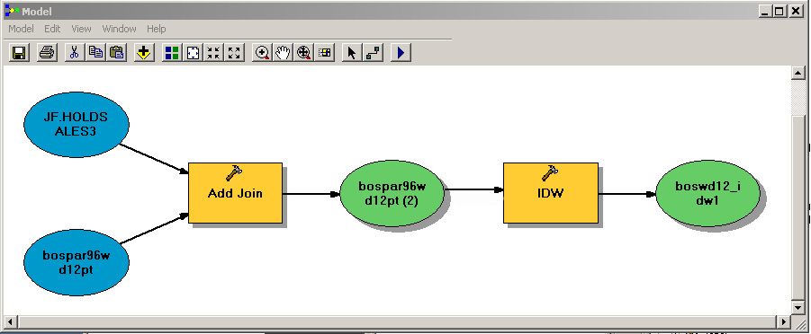
Review the ArcGIS help files regarding Model Builder and reread the 'Model Builder' notes in latter part of Lab #7 of the introductory GIS class (11.188), http://web.mit.edu/11.188/www14/labs/lab7/lab7.html. Then, create a new 'model' that results in a diagram with the IDW-averaging steps shown below. The example in the diagram shows Boston Ward 12 instead of East Boston and jf_holdsales3 instead of jf_holdsales4, but the steps are the same. That is, your model joins the holdsales4 table to ebos_centroids.shp and then uses the inverse distance weighted operation (IDW) to interpolate a housing value for each parcel.
Figure 2. Sample Model Builder flow chart.
There are several ways to build the flow chart, but you will probably find it most convenient to start building the model by dragging and dropping the appropriate operations from the Toolbox menu into the model builder flow chart window and then specifying the appropriate input data and parameters. Don't try to connect to Postgres from within Model Builder. 'Add' the table from Postgres(e.g., holdsales4) into your ArcMap session in the usual way (exporting and importing as a csv) and start the Model Builder diagram with the 'join' step that joins holdsales4 to the parcel centroid shapefile. Also, note that Model Builder uses the spatial analyst tools in ArcToolbox, which are a bit different from those used above from the 'Spatial Analyst' menu. In particular, you will need to set the desired raster analysis settings for ArcToolbox by right-clicking 'ArcToolbox,' choosing 'raster analysis setting,' and (once again) setting your grid cell size and mask, and choosing 'Processing Extent" to set the box within which calculations are done. Note that, for the ArcToolbox settings, you can set the extents to match those of another layer only if that layer is a raster grid (not a shapefile). Also, Right-clicking on 'ArcToolbox' to set 'environments' in the ArcToolbox window gets you to the same settings as choosing 'Geoprocessing / Environments' from the main ArcMap menus.
When using ArcToolbox, be aware that, on some WinAthena machines, you may get error messages indicating 'script' errors when trying to set parameters and environment variables for items in the flow chart. Just click 'yes' to continue and eventually you should get to the correct dialogue box. ArcGIS has some trouble on WinAthena machines with calling java scripts to process files resident in AFS lockers - for example to open the help files to the appropriate page. You can always open the ArcGIS help files separately from the Start/Programs/ArcGIS/ArcGIS-Desktop-Help... menu.
Part III: Lab Assignment
Most of the questions suggested above are simply to stimulate your thinking. Only a few items need to be turned in for this lab assignment. They are based on the revised SQL query that you used in Postgres to create xxx_holdsales4 for the sales that were considered arms-length. (You are welcome to redo the interpolation for the foreclosures - there were many in East Boston during this period! - but that is not required, and will produce distorted housing value estimates.). Turn in the following:
Home | Syllabus
| Lectures | Labs
| CRON | MIT
Created by Joseph Ferreira
Modified: March 2001-2004 by [thg] and [jinhua]; Last Modified:5 March 2018 [jf]