Deadlines
Useful links
channel.py -- BUG FIXED 9/21 virtual and IR channel interface
im1d.py -- image functions
brobot.png -- image
mandril.png -- image
lab1.py -- lab1 functions
lab2.py -- support and testing code for Lab #2
lab2_0a.py, lab2_0b.py -- files for Task #0
lab2_1.py -- template for Task #1
lab2_2.py -- template for Task #2
lab2_3.py -- template for Task #3
lab2_4.py -- template for Task #4
lab2_5.py -- template for Task #5
lab2.zip -- zip file containing lab 2 files
Numpy docs,
tutorial,
examples
Matplotlib.pyplot
reference,
tutorial
Instructions
See Lab #1 for a longer narrative about lab mechanics. The 1-sentence version:
Complete the tasks below, submit your task files on-line before the deadline, and sign-up with your TA for a check-off interview.
As always, help is available in 32-083 (see the Lab Hours web page).
Background and Goals
In this second 6.02 lab, you will be examining the problem of improving the quality of a communication channel. We hope that by examining this example problem you will become familiar with four key ideas in dealing with complicated systems. The first idea is that constructing the right picture can lend immediate insight in to a problem at hand (you will generate eye diagrams to help you determine the number of samples per bit needed for reliable transmission). The second idea is that the powerful techniques for analyzing linear time-invariant (LTI) systems can be brought to bear on non-LTI systems, provided the non-LTI system can be processed so that its behavior appears to be LTI (you will process the IR channel so that it looks like an LTI system). The third idea is that if one understands how a system corrupts a signal, one can reconstruct the uncorrupted signal from the corrupted signal, though noise makes perfect reconstruction impossible (you will use deconvolution to compensate for noise-free and noisy LTI channels). Lastly, we hope to familiarize you with the idea of creating new systems by composing together simpler systems (you will use Python classes to generate callable objects that create virtual channels from the composition of a basic channel with techniques for processing that channel).
In this lab you will use all the above ideas to demonstrate the impact on the eye diagram of using deconvolution to compensate for channel behavior. But please understand that the idea of unraveling system behavior is a far more general technique. Whether the problem is compensating for telescope or microscope nonidealities in images for astronomy or biological applications, or generating interpretable pictures from MRI signals in medical imaging, or reconstructing the original audio from turn of the century recordings, or estimating position from sensor data, the fundamental concept is the same. If you understand the system that relates the data you collect to the information you want, you can unravel the impact of the system and get at that information. BUT, noise will always make that process more difficult, and may make it impossible. If perfect reconstruction were possible in the presence of noise, there would never have been a space mission to fix the Hubble telescope.
Task 0: Performance issues in Python (0 points)
In this and a number of subsequent labs, you will be writing Python programs that transfer images represented as sequences of voltage samples. As noted in Lab 1, digitally transmitting even a small 64x64 pixel image can result in the generation of nearly a million voltage samples, so program efficiency can be an issue. In this zeroth task, you will examine the performance of two implementations of the bits_to_samples function used in Lab 1, both to remind you of how bits are represented using voltage samples when transmitting over channels, and to familiarize you with the fact that certain approaches to implementing algorithms in Python can have severe performance implications. The file lab1.py that you downloaded for Lab 1 included a function that generated a sequence of voltage samples from sequence of bits,
voltage_samples = bits_to_samples(bits,
                                samples_per_bit,
                                npreamble=0,
                                npostamble=0,
                                v0 = 0.0,
                                v1 = 1.0,
                                repeat = 1)
samples_per_bit -- how many voltage samples to output for each message bit. So total number of samples output for one repitition is npreamble + samples_per_bit*len(bits) + npostamble, where npreamble and npostample are described below.
Note, the rest of the arguments are keyword arguments and have default values.
npreamble -- number of "0" samples to output before any of the message bits are transmitted. See v0 keyword arg for value to be used.
npostamble -- number of "0" samples to output after all the message bits have been transmitted. See v0 keyword arg for value to be used.
v0 -- floating point voltage to use when generating samples for "0" bits (repeated samples_per_bit times).
v1 -- floating point voltage to use when generating samples for "1" bits (repeated samples_per_bit times).
repeat -- an integer specifying how many times to repeat the sequence of preamble samples, message samples, and postamble samples.
The default value for each keyword argument (i.e., the value used if the caller doesn't explicitly specify a value) is chosen so that no keyword arguments need be supplied unless the user is trying to do something out of the ordinary.
def bits_to_samples(bits,samples_per_bit,
             npreamble=0,
             npostamble=0,
             v0 = 0.0,
             v1 = 1.0,
             repeat = 1):
    """ generate sequence of voltage samples:
          bits: binary message sequence
          npreamble: number of leading v0 samples
          npostamble: number of trailing v0 samples
          samples_per_bit: number of samples for each message bit
          v0: voltage to output for 0 bits
          v1: voltage to output for 1 bits
          repeat: how many times to repeat whole shebang
    """
    # Default to all v0's
    samples = [v0]*(npreamble +
                    len(bits)*samples_per_bit +
                    npostamble)
    index = npreamble
    one_bit_samples = [v1]*samples_per_bit
    for i in range(len(bits)):
        next_index = index + samples_per_bit
        if bits[i] == 1:
            samples[index:next_index] = one_bit_samples
        index = next_index

    return samples*repeat
and lab2_0b.py:
def bits_to_samples(bits,samples_per_bit,
             npreamble=0,
             npostamble=0,
             v0 = 0.0,
             v1 = 1.0,
             repeat = 1):
    """ generate sequence of voltage samples:
          bits: binary message sequence
          npreamble: number of leading v0 samples
          npostamble: number of trailing v0 samples
          samples_per_bit: number of samples for each message bit
          v0: voltage to output for 0 bits
          v1: voltage to output for 1 bits
          repeat: how many times to repeat whole shebang
    """
    samples = [v0]*npreamble

    for i in range(len(bits)):
        vnext = v0 if bits[i] == 0 else v1
        samples = samples + [vnext]*samples_per_bit

    samples = samples + [v0]*npostamble

    return samples*repeat
In this task you will just collect data to use to answer the aab questions. You should determine which version of the bits_to_samples function runs faster and explain why (in your answers to the lab questions). You should try testing each version of the bits_to_samples function for sequences of bits that range in length from hundreds to hundreds of thousands. If you'd like to automate the collection of timing data, time.clock() returns a floating point number giving the current time expressed in seconds. There is no software to submit for this task.
The moral of the story is that when trying to code up processing steps on a large data set, it's good to pay attention to when storage is being allocated by the operators. Gratuitous reallocation of storage for million-sample arrays can led to frustratingly long runtimes.
Task 1: Generating eye diagrams (1 point)
Eye diagrams were introduced in lecture as a very effective way to visualize how a channel affects the sample sequences that pass through it. Recall that an eye diagram is just a plot of the channel output, but instead of creating a single plot of sample value versus time, we overlayed plots of the output waveform, where each overlay corresponds to a short segment of time. The length of a plot segment is typically three times the number of samples used to represent a single bit.
Write a Python function plot_eye_diagram that generates a new figure containing an eye diagram for the channel function passed as an argument:
In order to ensure that an eye diagram includes one complete period, along with the transitions from the previous and to the next bit periods, an eye diagram plot covers enough samples for three bit periods, or 3*samples_per_bit.
We have written a function plot_eye_diagram_fast that uses a fast trick for generating overlayed plots that exploits the way matplotlib's pyplot.plot command plots matrices. Our fast version is fast, and will be useful later, but is not very helpful for learning about eye diagrams. This fast version reshapes an array of received samples in to a two-dimensional matrix with a number of columns equal 3*samples_per_bit, and passes the transpose of this matrix to pyplot.plot.
In order to help you learn about eye diagrams, please write your plot_eye_diagram function so that it generates a bit sequence that is a merge of all possible 3 bit messages (you can use the all_bit_patterns function in the lab2_1.py template file), convert the bits to transmit samples, pass the transmit samples in to the channel passed to your function, and then plot the received samples by overlaying sets of 3*samples_per_bit samples. So that you can watch the eye diagram form, your function should wait for a press of the enter key after each plot of 3*samples_per_bit samples. The Python function raw_input will be helpful here. For example, raw_input('Press enter to continue'), would do the job.
lab2_1.py is a template file for this task:
import numpy
import channel
reload(channel)
import matplotlib.pyplot as p
import lab1
reload(lab1)
import lab2
reload(lab2)

p.ion()

def all_bit_patterns(n):
    # generate all possible n-bit bit sequences and merge into a single array
    message = [0] * (n * 2**n)
    for i in xrange(2**n):
        for j in xrange(n):
            message[i*n + j] = 1 if (i & (2**j)) else 0
    return numpy.array(message,dtype=numpy.int)


def plot_eye_diagram_fast(channel,plot_label, samples_per_bit):
    """
    Plot eye diagram for given channel using all possible 6-bit patterns
    merged together as message. plot_label is the label used in the eye
    diagram, Samples_per_bit determines how many samples
    are sent for each message bit.
    """

    # build message
    message = all_bit_patterns(6)

    # send it through the channel
    result = channel(lab1.bits_to_samples(message,samples_per_bit))

    # Truncate the result so length is divisible by 3*samples_per_bit
    result = result[0:len(result)-(len(result) % (3*samples_per_bit))]

    # Turn the result in to a n by 3*samples_per_bit matrix, and plot each row
    mat_samples = numpy.reshape(result,(-1,3*samples_per_bit))
    p.figure()
    p.plot(mat_samples.T)
    p.title('Eye diagram for channel %s' % plot_label)


def plot_eye_diagram(channel,plot_label, samples_per_bit):
    """
    Your, more educational, version of plot_eye_diagram.
    For given channel, you should generate a bit sequence made of
    all possible 3 bit messages (you can use the all_bit_patterns function
    above), and then plot the received samples by overlaying sets of
    3*samples_per_bit.  So that you can watch the eye diagram form,
    have the program stop for a press of enter after every 3*samples_per_bit
    plot The python function raw_input('Press enter to continue') will help.
    """

    pass # Your code here.


if __name__ == '__main__':

    # Create the channels (noise free with no random delays or padding)
    channel0 = channel.channel(channelid='0')
    channel1 = channel.channel(channelid='1')
    channel2 = channel.channel(channelid='2')

    # plot the eye diagram for the three virtual channels
    plot_eye_diagram(channel0,'0',samples_per_bit=50)
    plot_eye_diagram(channel1,'1',samples_per_bit=50)
    plot_eye_diagram(channel2,'2',samples_per_bit=50)

    # Create the channels with noise
    channel0 = channel.channel(channelid='0', noise=0.05)
    channel1 = channel.channel(channelid='1', noise=0.05)
    channel2 = channel.channel(channelid='2', noise=0.05)

    # plot the eye diagram for the three virtual channels
    plot_eye_diagram(channel0,'0n',samples_per_bit=50)
    plot_eye_diagram(channel1,'1n',samples_per_bit=50)
    plot_eye_diagram(channel2,'2n',samples_per_bit=50)
Once your function is working, experiment with the value of samples_per_bit for alll three software channels (in the next lab you will be using this function to help you with a design problem associated with the hardware IR channel). For each case, try to find the minimum value that produces an eye that is open enough to permit successful reception of the transmitted bits with and without noise. You should find that the minimum value is different for the three channels, and that a larger value is needed when there is noise. Once you feel you have the hang of eye diagrams, you can switch to using the faster version.
There are some lab questions (see link at top of page) associated with this task.
Task 2: Determining the unit-sample response of a channel (2 points)
In lecture we saw that the unit-sample response completely characterizes the effect of a channel on sequences of samples that pass through the channel. So, determining the unit-sample response of a channel is a handy way to model a channel and (as we'll see in later tasks). The unit-sample response is also useful in figuring out how to engineer the receiver to compensate for a channel's less desirable effects.
Please note: In order to instantiate a channel that is LTI, set channelid = '0' or '1' or '2', noise=0.0, and random_tails=0. The case of channelid = 'ir' will be treated in a subsequent task.
There are two common approaches for measuring the unit-sample response of a channel. One approach is straightforward but generates a signal that is difficult to detect using the 6.02 infrared communication channel, and a second approach that is a little more indirect, but generates signals that are easier to detect when using our hardware.
The most direct way to compute the unit-sample response, h[n], is to transmit a single sample that has the value 1.0, followed by many zero samples (NOTE: A SINGLE VOLTAGE SAMPLE, NOT A SINGLE BIT -- the bits_to_samples function is irrelevant when determining unit-sample response, use it and you will be assimilated). For example, a K-long sample sequence of a single 1.0 followed by zeros can be generated using numpy.array([1.0] + [0.0]*(K-1)). When this sequence is passed to a linear time-invariant channel, the sequence that is returned is the unit-sample response of the channel.
There is a problem with using the above approach to compute the
unit-sample response on a channel like the IR hardware.
The IR channel response to a single nonzero sample is so
small compared to the channel noise, that it can be difficult to
detect the beginning of the unit-sample response. An approach that
generates a larger signal that is more easily detected in the IR channel
is to first compute the step
response, where the step response is the result of transmitting a long
sequence of samples all equal to 1.0. Denoting the step response as
s[n], the unit-sample response is then related to the difference
between the step response and a one-sample-delayed step response, h[n]
= s[n] - s[n-1].
We suggest that you use the step response approach to computing unit-sample responses, but there is another small complication. Formally, the unit-sample response (USR) is specified for an infinite number of samples. For all practical purposes, the USR will be so close to zero after a modest number of samples, that a USR-based model of a channel will still be quite accurate even if we truncate the response to a finite number of samples (as long as the samples beyond the truncation point are sufficiently close to zero). To find a reasonable point to truncate a USR, note that you'll need to start with a USR that is much longer than the truncated USR.
For this task, write a Python function unit_sample_response that returns a truncated sequence of samples that corresponds to the unit-sample response of the specified channel:
If tol > 0, the response sequence should be truncated at an index K if the maximum magnitude of the values of the samples from index K+1 to max_length are smaller than tol times the largest magnitude sample in the unit-sample response. You may find that the numpy function numpy.nonzeros is useful for simplifying this task.
If tol = 0, the response sequence should be of length max_length.
lab2_2.py is a template file for this task:
# template for Lab #2, Task #2
import numpy
import matplotlib.pyplot as p
import channel
reload(channel)
import lab2
reload(lab2)

# turn on interactive mode, useful if we're using ipython
p.ion()


# arguments:
#   channel -- instance of the channel.channel class
#   max_length -- integer
#   tol -- float
#   pad -- integer
# return value:
#   a numpy array of length max_length or less
def unit_sample_response(channel,max_length=1000,tol=0.005,pad=50):
    """
    Returns sequence of samples that corresponds to the
    unit-sample response of the channel.  The unit sample response
    should be calculated by computing the difference between
    shifted step responses, where the number samples in the step
    response should be "pad" more samples than needed in the
    calculation of the unit sample response (this eliminates end
    effects). The voltage sample sequence representing the unit
    sample response should truncated to the smallest length such
    that the maximum magnitude of the truncated samples are
    smaller than than "tol" times the value is the largest
    magnitude sample in the unit sample response. Please make
    sure that if tol=0.0, then the return USR should have length
    equal to max_length.
    IMPORTANT: Please read the hints in the lab handout before starting.
    """
    pass # Your code here.

if __name__ == '__main__':
    # Create the channels (noise free with no random delays
    # or padding)
    channel0 = channel.channel(channelid='0')
    channel1 = channel.channel(channelid='1')
    channel2 = channel.channel(channelid='2')

    # plot the unit-sample response of our three virtual channels
    lab2.plot_unit_sample_response(unit_sample_response(channel0),
                                   '0')
    lab2.plot_unit_sample_response(unit_sample_response(channel1),
                                   '1')
    lab2.plot_unit_sample_response(unit_sample_response(channel2),
                                   '2')

    # when ready for checkoff, enable the following line
    #lab2.checkoff(unit_sample_response,'L2_2')
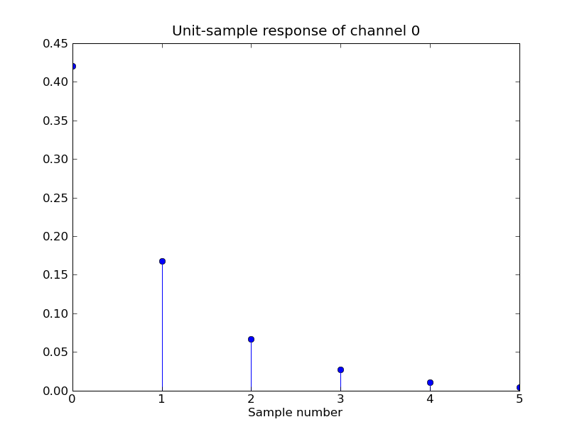
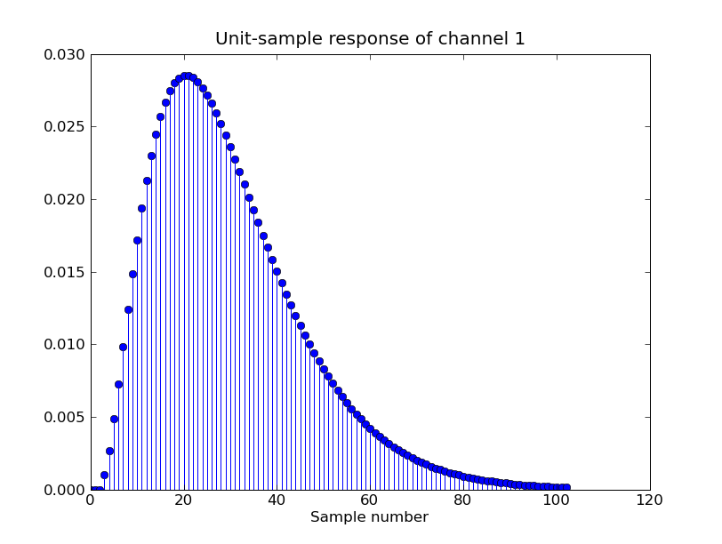
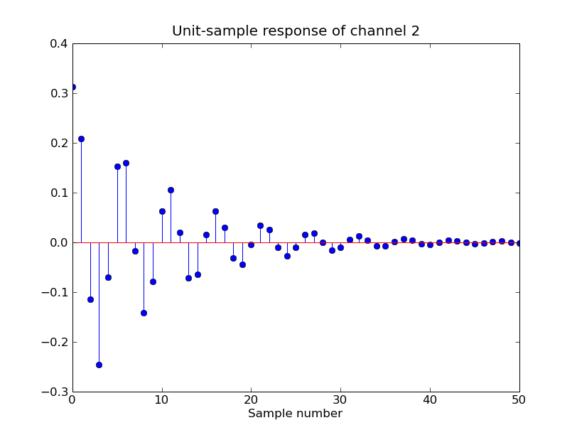
The test code uses your function to compute the unit-sample response of our three channels and plots the result. If your function is working correctly you should see something like
When you're satisfied with your implementation, enable the call to lab2.checkoff which will submit your code on-line.
There are some lab questions (see link at top of page) associated with this task.
Task 3: Predicting channel behavior using the convolution sum (1 point)
We also saw in lecture that given the unit-sample response we can compute the effect of the channel on an arbitrary input by performing the appropriate convolution sum.
Write a Python script that does the following for each of the three channels used in Task #2:
lab2_3.py is a template file for this task:
import numpy
import matplotlib.pyplot as p
import channel
reload(channel)
import lab1
reload(lab1)
import lab2
reload(lab2)
import lab2_2
reload(lab2_2)

p.ion()

# arguments:
#   usr -- numpy.array returned by unit_sample_response
#   mychannel -- instance of the channel.channel class
#   cname -- string used in plot title
#   samples_per_bit -- integer
# return value:
#   none
def compare_usr_chan(usr,mychannel,cname,samples_per_bit):
    """
    Transmit the bit sequence [1,0,1,0,1,0,1,0] using
    "samples_per_bit" samples for each bit through the "mychannel",
    and then compare the results to the results generated using
    convolution with the "usr" (unit sample response).  Generate
    a plot with three subplots: the samples received from the
    channel, the samples generated by convolution, and the
    difference between the two.   Use the string "cname" for
    the title of the plot.
    """
    pass # Your code here.


if __name__ == '__main__':
    # plot the unit-sample response of our three virtual channels

    # Create the channels (noise free with no random delays
    # or padding)
    channel0 = channel.channel(channelid='0')
    channel1 = channel.channel(channelid='1')
    channel2 = channel.channel(channelid='2')

    samples_per_bit=8
    compare_usr_chan(lab2_2.unit_sample_response(channel0),channel0,
                     "channel 0", samples_per_bit)
    samples_per_bit=30
    compare_usr_chan(lab2_2.unit_sample_response(channel1),channel1,
                     "channel 1", samples_per_bit)
    samples_per_bit=20
    compare_usr_chan(lab2_2.unit_sample_response(channel2),channel2,
                     "channel 2", samples_per_bit)

    # when ready for checkoff, enable the following line
    #lab2.checkoff(compare_usr_chan,'L2_3')
Notice that in our template, you must write the function compare_usr_chan(usr,mychannel,cname,samples_per_bit=8), where usr is the unit-sample response computed from task 2, the mychannel argument will be a channel instance just as before. The string cname should just be used for the title for the plots you must generate as described above, and we are sure you should know what samples_per_bit is by now.
There are some lab questions (see link at top of page) associated with this task.
Task 4: Unit-Sample Response for the IR Channel (2 points)
Random delays in the IR hardware channel's response mean that the IR channel is NOT time-invariant. In addition, the fact that the lowest signal level from the IR hardware is a little above 0.2 volts implies that the IR channel is also NOT linear. However, by including a calibration signal one can remove the delay and shift and scale the response of the received IR signal to create a system that is effectively linear and time invariant. In this task, you will do just that, and then use your results from Task 2 and Task 3 to demonstrate that you have succeeded.
Using a paper reflector in front of the IR hardware run your Lab #1, Task #1 code to see how the IR channel affects the transmitted signal. You'll see that the signal levels differ from the 0-1V signaling of the software channels, and that the timing of the received signal is shifted significantly from the timing of the transmit signal. Try running the Lab #1, Task #1 code with the reflector a couple of feet away from the board -- you should see that the signal levels fall off dramatically. It would be very useful to convert the actual signal levels back to the 0-1V signaling expected by the processing routines you created above.
If you examine the template below for this task, you will notice that we have written the initialization routine for a scaled_ir class, one that includes the creation of a numpy array mark. This mark should be prepended to a sequence of samples sent to the IR channel, so that the scale and delay of the received samples can be determined. In addition, we have written the member function find_start(self, scaled_data), which uses the result of convolving the scaled received data with a zero-averaged version of mark to determine which sample index in the received data corresponds to the transmitted message. NOTE THAT THERE IS A PARAMETER offset THAT MUST BE CALIBRATED BEFORE YOU CAN USE THE find_start function. If you uncomment the plotting in the find_start function, you can better understand what is going on. You should be able to explain how this routine works during the lab interview. In particular, you should be able to explain why the value you determined for this offset was negative.
lab2_4.py is a template file for this task:
import numpy
import matplotlib.pyplot as p
import channel
reload(channel)
import lab1
reload(lab1)
import lab2
reload(lab2)
import lab2_2
reload(lab2_2)
import lab2_3
reload(lab2_3)

p.ion()

def plot_with_title(data,title):
    """
    Create a new figure and plot data using blue, square markers.
    """
    p.plot(data)   # line plot
    p.title(title)
    p.xlabel('Sample data')
    p.ylabel('Voltage')
    p.grid()


class scale_ir:

    def __init__(self, mark_size=800):
        # Get the ir channel
        #self.irchannel = channel.channel(channelid='2',random_tails=100)
        self.irchannel = channel.channel(channelid='ir')

        # Create a 0s, 1s, 0s mark to prepend data
        self.mark = numpy.zeros(3*mark_size)  # Create 0s 0s 0s + pad
        self.mark[mark_size:2*mark_size] = 1  # Set to 0s 1s 0s + 0 pad


    # arguments:
    #   input -- numpy.array of voltage samples to be transmitted
    # return value:
    #   numpy.array of received voltages from ir channel, scaled
    #   and offset so that the values range from 0 to 1
    def __call__(self,input):
        # Should prepend "mark" to the "input", send the result
        # through the ir channel (hardware is needed), and then
        # process the received data.  The mark samples should be
        # used to determine shifting and scaling for the channel,
        # so that the returned signal is between zero and one,
        # regardless of the ir hardware reflector position. The
        # mark should then be removed, along with any leading
        # zeros. You can use the find_start function to help you with
        # this, but you will need to calibrate offset!

        return input # Your code here


    def find_start(self, scaled_data):
        # Make sure the data is scaled correctly
        mind = numpy.min(scaled_data)
        maxd = numpy.max(scaled_data)
        assert max([abs(mind), abs(maxd - 1.0)]) < 0.05, "Unscaled data!"

        # Compute a version of the mark that has zero average value.
        zero_avg_mark = self.mark - numpy.average(self.mark)

        # Convolve the zero-averaged mark with the scaled_data
        # What happens if you convolve the original mark with a sample
        # sequence whose sample values are all one? How does the result of
        # this convolution change if you replace "mark" with "zero_avg mark?
        convolved_with_data = numpy.convolve(zero_avg_mark, scaled_data)

        # These two lines return the index of the first sample
        # in convolved_with_data that is equal to convolved_with data's
        # maximum value.  What is import about the sample index where
        # convolved_with_data achieves its maximum?
        max_conv = numpy.max(convolved_with_data)
        start_index = numpy.nonzero(convolved_with_data == max_conv)[0][0]

        """
        p.figure
        p.plot(convolved_with_data[0:len(scaled_data)])
        p.plot(scaled_data*max_conv)
        p.axvline(x=start_index)
        """
        # Start index is consistently to large by a particular amount (Why?)
        # Determine the offset by experiment.
        offset = 0
        assert offset != 0, "Offset is zero!  You must calibrate it."
        start_index += offset
        #print "start index", start_index
        return start_index


if __name__ == '__main__':

    # Create scaled_ir channel
    myir = scale_ir()
    my_un_ir = channel.channel(channelid='ir')

    # Compare the scale_ir channel to the non-scaled ir channel
    bits = [1,0,1,0,1,0,1,0]
    samples_per_bit = 500
    test_samples = lab1.bits_to_samples(bits,samples_per_bit,npostamble=100)
    out_samples = myir(test_samples)
    out_un_samples = my_un_ir(test_samples)


    # Plot the comparison for testing
    p.figure()
    p.subplots_adjust(hspace = 0.6)
    p.subplot(311)
    plot_with_title(test_samples,"Input")
    p.subplot(312)
    plot_with_title(out_un_samples,"Unscaled and Shifted")
    p.subplot(313)
    plot_with_title(out_samples,"Scaled")

    #Uncomment when ready to test
"""
    # Compute the usr and average
    ausr = lab2_2.unit_sample_response(myir,max_length=400,tol=0.0)
    for i in range(9):
        ausr += lab2_2.unit_sample_response(myir,max_length=400,tol=0.0)
    ausr /= 10.0

    # Plot the unit_sample response
    lab2.plot_unit_sample_response(ausr, "scale_ir")

    # Demonstrate the ability to predict
    lab2_3.compare_usr_chan(ausr, myir, "scale_ir",samples_per_bit=100)


    # when ready for checkoff, enable the following line
    # BUT BE SURE You still connected to the IR system you tested.
    #lab2.checkoff(scale_ir,'L2_4')

"""
For this task, please write the __call__(self,input) routine for the class scaled_ir. The routine should prepend the self.mark in front of the sequence of samples, input, and then send the resulting sequence through the channel instance self.irchannel. Using what you know about the mark, shift and scale the received sample values so that they all lie between zero and one. Then use your calibrated find_start function to strip off any leading junk and the mark. Finally, the routine should return the processed sequence of samples as a numpy array of the same length as input.
Note that the mark must be prepended to every message sent across the IR channel, to ensure that the maximum and minimum signal levels of the IR channel are achieved on every transmission. This ensures that the scaling depends only on the channel, and not on the particular data being sent.
Also note that IR channel will return unpredictable junk samples before and after the transmitted data, so you'll have to think carefully about why a calibrated version of find_start should almost always work.
HINTS: The IR channel is "slow", i.e., transitions between low and high signal levels take multiple sample times to complete. What do you think that means about the sign of offset in find_start
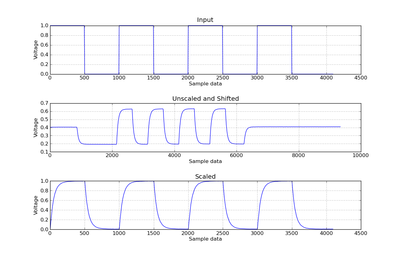
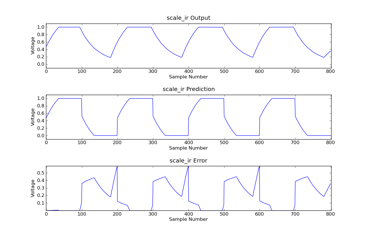
The provided template uses your results from Task 2 to generate a comparison plot between the scaled_ir and unscaled ir channel. If your code is working, you should see a plot like the one below.
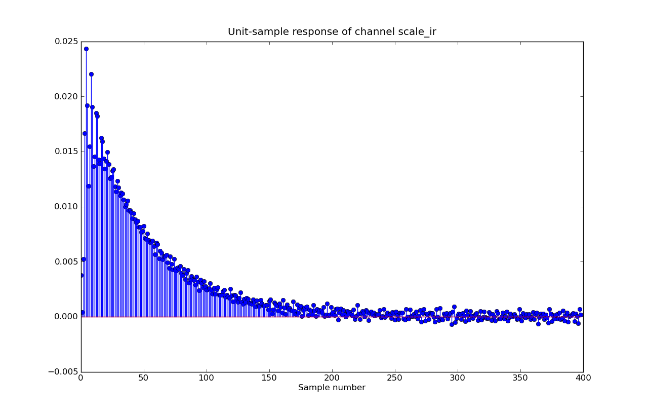
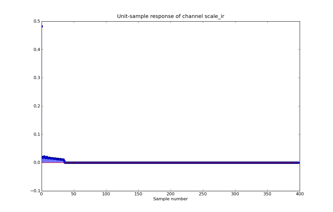
The provided template also generates a unit-sample response for the scaled_ir channel by averaging ten unit-sample responses. The averaging helps reduce the impact of IR channel noise, but does not eliminate it. In the lab questions you will be asked to explain why tol is set to 0. The template then uses your results from Task 3 to demonstrate that convolving with the averaged unit-sample response for the IR channel does correctly predict the behavior of the scaled_ir channel.
To demonstrate that you've completed this part, you should generate plots of the unit-sample response and the comparisons that look something like the following.
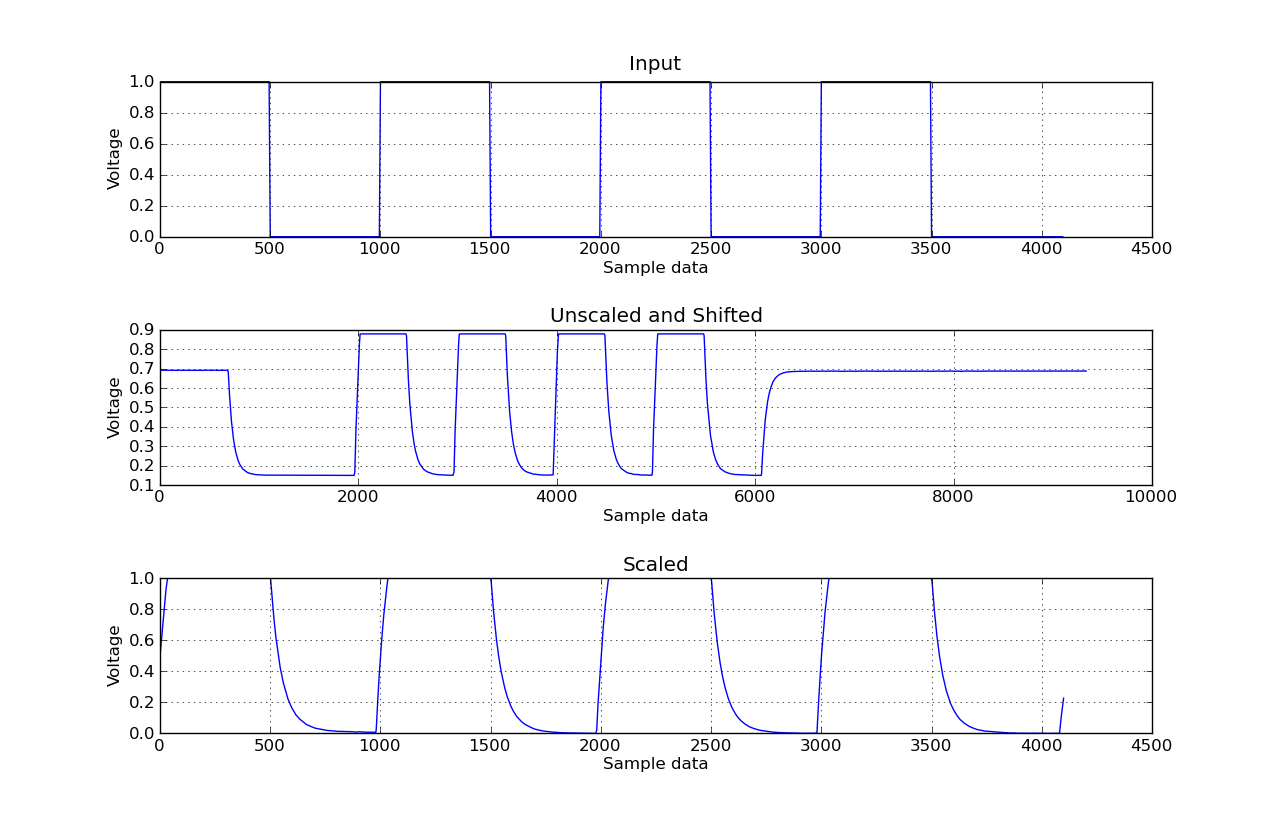
WARNING: DO NOT PLACE THE PAPER REFLECTOR CLOSER THAN SIX INCHES FROM THE IR BOARD. If the reflector is too close, the IR optical detectors will get saturated and destroy any hope of generating an LTI representation. If your comparison plots have very flat tops, or if your unit-sample response computation produces a peak and then drops to exactly zero, like in the pictures below, then you should move the paper reflector further away. Otherwise, your convolved result will not match the received result (like in the third figure below).
IF YOUR RESULTS LOOK LIKE THE PLOTS BLELOW YOUR REFLECTOR IS TOO CLOSE!
Task 5: Deconvolution (3 points)
In lecture we talked about deconvolution, an approach to reconstructing the signal at the input to the transmission system by looking at the transmission channel's output (Y) and using the channel's unit-sample response (H).
In particular, we showed that the sequence W would be a reconstruction of the input sample sequence X if W satisfied the difference equation
y[n] = h[0]w[n] + h[1]w[n-1] + ... + h[K]w[n-K].
where Y is the sequence of channel output samples and the unit-sample response H is zero after some number of samples, i.e., h[n] = 0 when n > K.
We can rearrange this equation to solve for w[n]:
w[n] = (1/h[0])(y[n] - h[1]w[n-1] - ... - h[K]w[n-K]).
Since you are given Y, and since you know w[n] = 0 for n < 0, you can solve the above equation for w[0] given y[0], then for w[1] given w[0] and y[1], and so on:
w[0] = (1/h[0])(y[0])
w[1] = (1/h[0])(y[1] - h[1]w[0])
...
You will have to think carefully about how to modify this simple "plug and chug" strategy when the leading values of H (h[0], h[1],..) are zero.
lab2_5.py is a template for your Task 5:
# template for Lab #2, Task #5There are three parts to this deconvolution task:
import numpy,random
import matplotlib.pyplot as p
import channel
reload(channel)
import im1d
reload(im1d)
import lab2
reload(lab2)
import lab1_1
reload(lab1_1)
import lab2_2
reload(lab2_2)
# turn on interactive mode, useful if we're using ipython
p.ion()
# arguments:
# samples -- numpy array of received voltage samples
# h -- numpy array as returned by unit_sample_response
# return value
# numpy array of deconvolved voltage samples
def deconvolver(samples,h):
"""
Take the samples that are the output from a channel (y), and
the channel's unit-sample response (h), deconvolve the
samples, and return the reconstructed samples. Be sure the
length of the reconstructed samples is the same as the length
of the input samples.
"""
#pass # your code here...
if __name__ == '__main__':
# Create two noise free channels
mychannel1 = channel.channel(channelid='1',noise=0.0)
mychannel2 = channel.channel(channelid='2',noise=0.0)
# Compute the channel unit sample responses of the
# noise-free channels
h1 = lab2_2.unit_sample_response(mychannel1)
h2 = lab2_2.unit_sample_response(mychannel2)
# Generate a sequence of test samples
samples = numpy.sin(2*numpy.pi*0.01*numpy.array(range(100)))
samples[0:len(samples)/2] += 1.0
samples[len(samples)/2:] += -1.0
maxs = max(samples)
mins = min(samples)
samples -= mins # Make samples positive
samples *= 1.0/(maxs - mins) # Scale between zero and one
# Test deconvolver
lab2.demo_deconvolver(samples,mychannel1,h1,deconvolver)
lab2.demo_deconvolver(samples,mychannel2,h2,deconvolver)
"""
#(Uncomment when ready to test) on a bigger data set.
# Read in a .png image as array of greyscale values
# between 0.0 and 1.0
image1 = im1d.im1dread("mandril")
image2 = im1d.im1dread("brobot")
lab2.demo_deconvolver(image1,mychannel1,h1,deconvolver,
images=True)
lab2.demo_deconvolver(image2,mychannel2,h2,deconvolver,
images=True)
"""
# when ready for checkoff, enable the following line
#lab2.checkoff(deconvolver,'L2_5')
Note the unit-sample response of one of the channels has leading zeros (h[0] will be zero). Your deconvolver code should handle this case correctly. When you're happy with the implementation, enable the call to lab2.checkoff.
There are some lab questions (see link at top of page) associated with this task.
Task 6: The real eye-opener (2 points)
What is the impact of using deconvolution on the number of samples needed per bit for channels '1' and '2', at least in the noise free case? For this task, consider creating a deconvolved channel class (like the scaled_ir class) so that you can use results from Tasks 1, 2, 3 and 5 to generate the eye diagrams for plain channels '1' and '2', and compare them to the results from deconvolved channels '1' and '2'.
There is no template for this task, but you should be able to generate the eye diagrams to answer the questions and to show during your check-off interview.