It is now time
to talk a bit about the mathematical properties of Brownian motion.
First of all, it
has the so-called Markov property. This means that the future is determined by
only knowing the present position and not the history of the walk. Put simply, Brownian motion forgets its past.
Two further very
important properties are the following
Ø
It is
a nowhere differentiable function!
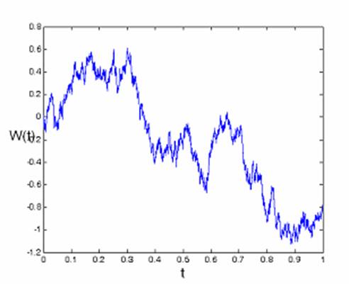
This sound very peculiar. Can we see it somehow? Let’s create a random walk,
given in the following figure, where the position is called W(t), “t” being the
time.
How can we see
if there is a derivative to that? We must first approximate the derivative, so
that we can implement it on a computer. This can be done by taking  .
.
We know that the
definition of a derivative is taking the above as the limit of dt goes to 0.
Know we will just choose a small enough dt, for example dt=0.0002 and here is
the result
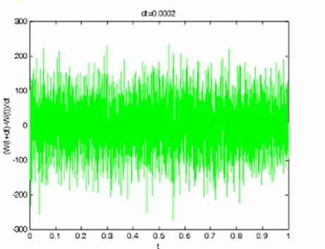
We can see that
this is nothing like a well defined function!
Ø
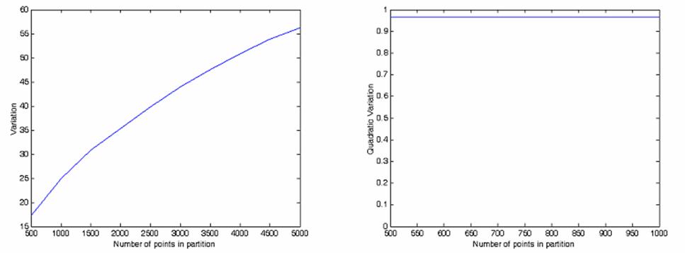
It
is a function with infinite variation, but bounded quadratic variation.
I admit that
this sounds puzzling, so we will just present the results as the two following
figures, without further comments.
All this was
done for Brownian motion in one dimension. What about higher dimensions?
As we have seen
from the “chessboard example”, in higher dimensions we can treat Brownian
motion as 1-dimensional Brownian motion in each dimension separately!