Since we are all
sitting in front of computer screens, it is worth talking a bit about how
Brownian motion is studied in these machines!
Technically, one
can say that the numerical construction of a Brownian motion can be done in two
ways
·
As a
scaled random walk
·
In terms
of random Fourier series
WHAT???
OK, you are
right to be complaining, this sounds confusing!
Let’s just try
to understand the first of the two alternatives.
I’ll first give
you the definition and then the recipe and the results.
Definition:
Brownian motion
may be considered as a scaled version of the usual random walk on the lattice
with probability ½ to make aleft move and ½ to make a right move. In the limit where
the jumps take place every dt and the length of the jumps are dx, where dt goes
to 0, dx goes to 0 AND dx2/dt goes to 1, using (something called)
Central Limit Theorem, we may show that this random walk tends to the Brownian
motion.
OK, but how do
we actually do it?
The following
short algorithm solves this problem
for i=1:N
dW(i)=sqrt(dt)*rand
W(i+1)=W(i)+dW(i)
end
Let’s see what
the algorithm means: dW(i) contains the increments of the Brownian motion, rand
is a random number and W(i) contains the Brownian motion at time interval “i”.
Now let’s see
what we get!
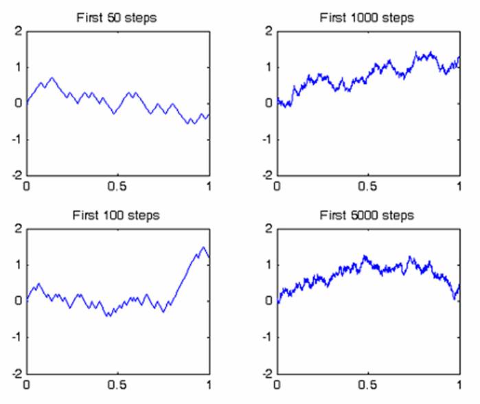
Voila!