Brownian motion and random walks
On this page, you will learn about random walks and Brownian motion. We will use this in the next couple of pages to explain some models of randomly growing surfaces.
In the introduction, we said that we wanted to study randomly growing surfaces, but what does that mean, exactly? What does it mean for something to be random and how can a surface grow randomly? To answer these questions, we will start more carefully and talk about random walks of particles.
Imagine a gas molecule in the air: it moves around on its own until it hits another gas molecule which makes it change direction. Since there are so many gas molecules in the air, it will constantly bump into other molecules (roughly \(10^{14}\) hits per second - that equals the total number of Google searches performed worldwide during 79 years!) and it will be just as likely to be hit from another particle on the left as it will be to be hit on the right. The bumps therefore cancel each other out, so after a long time interval, it will barely have moved at all, even though it makes really quick jerks all the time. The way the gas molecule moves will turn out to be important to studying randomly growing surfaces, so we will keep going on this track for a while!
Random walks
First, we want to try to model how this gas molecule moves in the simplest possible way, and you will explore one of these models in the following exercise.
Exercise: random motion from coin tosses and dice rolls.
In this exercise, you will generate two different random motions on your own.
a): We start with a one-dimensional motion. Draw a coordinate system with time \(t\) on the horizontal axis, and height \(h\) on the vertical axis. Mark the origin. Now, flip a coin. If heads, mark a point one step ahead and one step above the previously marked point. If tails, mark a point one step ahead and one step below the previous one. Continue this for a while and draw the resulting graph.
b): What is the average of \(h\), as a function of time? Calculate this in a table.
c): What is the average of \(h^2\), as a function of time? Calculate this in a table.
d): What way do you think would be a good way of measuring how far the random walk has gone from the origin? Is the average of \(h\) a good quantity? Is the average of \(h^2\) better or worse?
e): Next, you will draw a two-dimensional random walk. Draw a chessboard pattern around the origin, and roll a die. If you get a \(1\), mark the square to the left of the previous square. If \(2\), mark the square below the previous one. If \(3\), mark the one to the right, and if \(4\), mark the one above. If you get \(5\) or \(6\), roll again.
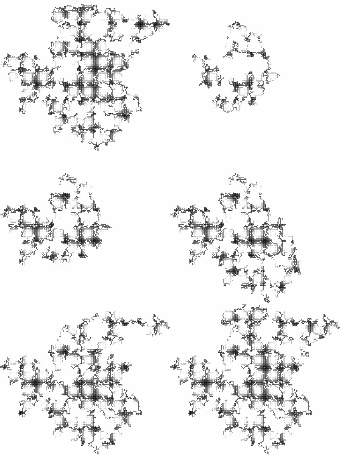
This is a very simple model of how the gas molecule can move, but it is also close to reality! To see a larger example, the following is a two-dimensional random walk generated in the same way as the exercise.

A (bigger) two-dimensional random walk
Even though the motion is quick and jerky, the particle doesn't get very far for large times - just like for gas molecules! Maybe we are on to something!
Brownian motion
Real gas molecules can move in all directions, not just to neighbors on a chessboard. We would therefore like to be able to describe a motion similar to the random walk above, but where the molecule can move in all directions. A realistic description of this is Brownian motion - it is similar to the random walk (and in fact, can be made to become equal to it. See the fact box below.), but is more realistic. In the beginning of the twentieth century, many physicists and mathematicians worked on trying to define and make sense of Brownian motion - even Einstein was interested in it!
In-depth fact: imagine a random walk on a chessboard, where the distance between the center of the squares is \(1/N\). As \(N\) tends to infinity, a random walk on this chessboard tends to a Brownian motion. To learn more about this, see the references on the ‘‘central limit theorem’’ below.
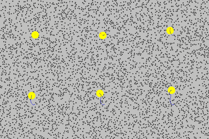
To get started, the following is a simulation of a gas, and one particle is marked in yellow. Its path describes a Brownian motion \(B_t\) at time \(t\).

Gas molecule (yellow) describing Brownian motion
Now, Einstein realized that even though the movements of all the individual gas molecules are random, there are some quantities we can measure that are not random, they are predictable and can be calculated. One such quantity is the density \(\rho\) of the gas molecules. Einstein showed that the density satisfies a differential equation
\[ \frac{\partial \rho}{\partial t} = D\frac{\partial^2 \rho}{\partial x^2}, \]
called the diffusion equation, and where \(D\) is the diffusion coefficient that can be calculated. This is an equation that can be solved, so we are able to predict something with certainty from a random model - this is an example of the strategy that is used in statistical mechanics. Einstein's equation showed that diffusion processes, for instance seeing a drop of ink spread out in water, are caused by Brownian motion - the question we will ask for the next pages is: can Brownian motion explain also other random phenomena?
Exercise: Code your own Brownian motion! If you have learned a programming language, find out how to generate a normally distributed number with variance \(s\) in that language. In Python, for instance, this is done by
the commands
import random
randomNumber = random.gauss(0, \(s\))
To generate a Brownian motion, follow the following steps:
we want to generate a brownian motion at times \(0, 0.1, 0.2, … , 1\). \(B_0\) is defined to be \(0\).
By definition, \(B_{0.1} - B_0\) is normally distributed with variance \(0.1\), so generate one such number and let that be the value of \(B_{0.1}\).
\(B_{0.2} - B_{0.1}\) is again normally distributed with variance \(0.1\), so generate one such number and add that to \(B_{0.1}\) to get the value of \(B_{0.2}\).
Write a program that continues this procedure!
Challenge question: Write a program that calculates Brownian motion at any set of times!
Further reading:
J. Matson, ‘‘Crowd Forcing: Random Movement of Bacteria Drives Gears’’, https://www.scientificamerican.com/article/brownian-motion-bacteria/.
Feynman, ‘‘Feynman Lectures on Physics’’, http://www.feynmanlectures.caltech.edu/I_41.html.
Central Limit Theorem, https://en.wikipedia.org/wiki/Central_limit_theorem.