On this page, we will start exploring some models for random surface growth. Along the way, we will discuss correlation functions, universality and stochastic differential equations.

Now that we have a better understanding of what it means for something to be random, we can start to explore some models the physicists and mathematicians use to describe random surface growth. Some of these models have been investigated for 20-30 years, and some are still being explored, so hopefully you will get a sense of some topics that are at the cutting edge of science right now!

Correlation functions

Like we talked about in the introduction, the questions we can answer about random models are different from the ones you might have seen in physics before. One main question that we can ask about all the models we will consider is how far the presence of a particle affects other particles around it. This is measured by the so called correlation function at distance \(r\), which we will write \(C(r)\). \(C(r)\) measures how a quantity \(X\) (such as the density of bacteria, the presence of a crystal particle, depth of snow coverage et.c.) varies over the whole system (bacterial colony, crystal, city), compared to the quantity \(X\) at points that are a distance \(r\) away. It is defined by

where the integral runs over the whole system. Typically, we will see that the correlation function behaves as a power law, i.e. \(C(r)\) is proportional to \(r^{\eta}\) for some real number \(\eta\). We will see later that this indicates that the system is scale-invariant and behaves like a fractal (more about this on the next page!).

A high value of the correlation function means that different parts of the system tend to vary together, so the system is very ordered. A low value of the correlation function means that different parts of the system behave differently, so it is not ordered.

When discussing the models below. we will mention the correlation functions of the systems, to see how much order there is in each system.

Universality

What does liquid helium and fish flocking in the ocean have in common? The answer might seem to be ‘‘not much’’, but it turns out that they actually behave very similarly - so much so that physicists use the same tools to study both of these systems! This is an instance of universality in physics, that the same principles and behaviors for one system will be applicable also to a completely different system. This is because their correlation functions behave in the same way: they have the same exponents in their expressions for \(C(r)\)! This means that by studying one system (maybe the easiest one), we can learn much also about other systems.

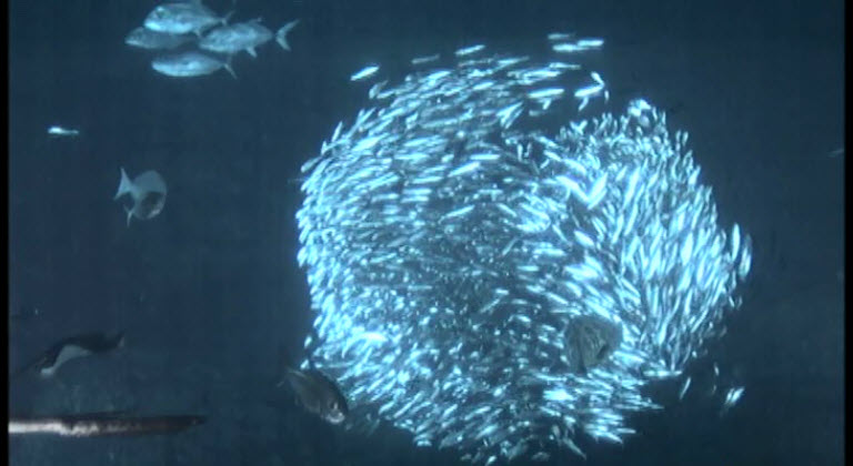
Schools of fish flocking together

Liquid helium

There are more exponents than the one for the correlation function that are included in the concept of universality. There are many so called critical exponents in statistical mechanics, that determine much of how a system behaves. Think of boiling water on the stove: the water goes from a liquid phase to gas in a phase transition. Another example would be magnets: if you cool a magnetic material below a certain threshold Curie temperature \(T_c\) (\(c\) for ‘‘Curie’’ or ‘‘critical’’), it will become spontaneously magnetic - and strongly so! Watch a demonstration in the video below.

Cooling a ferromagnetic material below the Curie point

This is used in for instance magnetical storage to erase data! After cooling to a temperature \(T < T_c\), the magnetization will be proportional to \((T_c-T)^{\beta}\), for some real number \(\beta\). In the same way, the heat capacity of the material will be proportional to \((T_c-T)^{\alpha}\) for some real number \(\alpha\). These numbers \(\alpha , \beta , \eta\) are the critical exponents and turn out to be the same also in different settings, for instance for superfluids, and different physical systems can be divided into universality classes which have the same values of these exponents. Even though they are different, this means that they will all have similar behaviors.

Diffusion limited aggregation

Let's imagine a colony of bacteria forming in a liquid. The bacteria are all flowing around on their own – just like the gas molecules on the previous page – so we can model each bacterium as doing its own Brownian motion. That is, until they bump into the part of the colony that has already been formed - then they stick together, and will no longer move around.

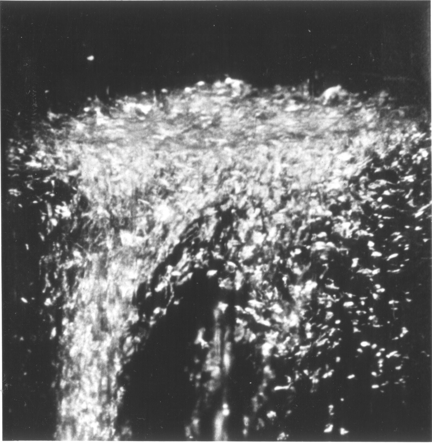
This is a simple model called diffusion limited aggregation, but why should it explain the intricate patterns that we saw in the pictures in the introduction? Well, let's try and see what happens. The following is a simulation of diffusion limited aggregation - click the button and see what happens! You can adjust the number of particles in the simulation, as well as the size of the box by dragging the sliders.
Note: if the browser starts reacting slowly after running the simulations, refresh the page!

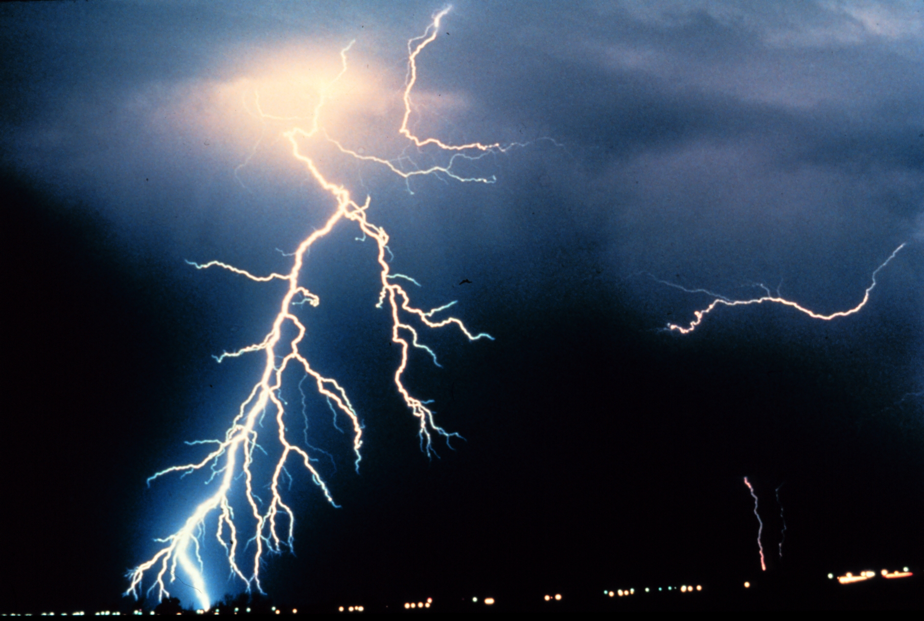
Lightning strike similar to diffusion limited aggregation

These are the same patterns that scientists observe in nature! These branchy and vessel-like structures can be found in many different places, like lightning strikes, blood vessels in the lung and the growth of ions during electrolysis. It has even been used to model how wounds in the human skin heal!

Note also that the surface that is grown in the simulation looks very treelike - it is actually a fractal, which we will discuss more on a following page. If you ran the simulation many times, you might have noticed that the simulated surface looked slightly different each time - all the same, it is still possible to calculate some quantities that characterize the surface. One of these is the correlation function, and one other quantity we will encounter later is the fractal dimension of the surface. In the original paper describing diffusion limited aggregation, the authors measured the correlation function of the simulations and found a value of \(C(r)\) proportional to \(r^{-0.343 \pm 0.004}\).

In three dimensions, diffusion limited aggregation looks like in the following simulation:

Eden-Richardson growth model

Often in biology, there is a large number of parameters that determine how a biological system evolves and it is easy to get overwhelmed with all the details. As a representative example, the following (taken from https://arxiv.org/pdf/1606.00463.pdf) is a system of partial differential equations that model how certain chemicals (denoted by F, B, R, K, P, L below), are secreted in response to simulation for biological cells:

\[ \begin{align} F_t(x,t) +vF_x(x,t) &= - k_1(R(x,t)-B(x,t))F(x,t) +k_2B(x,t) \\ B_t(x,t) &=k_1(R(x,t)-B(x,t))F(x,t)-k_2B(x,t) \\ R_t(x,t) &=a_0-b_0R(x,t)-c_0B(x,t) \\ K_t(x,t) &=b_1B(x,t)-a_1K(x,t)P(x,t) \\ P_t(x,t) &=b_2K(x,t)-a_2P(x,t) \\ L_t(x,t) +vL_x(x,t) &= bs + b_3K(x,t) \\ \end{align} \]

This is pretty complicated!! When possible, it is therefore much better if you can find as simple a model as possible describing the system you are interested in, and we will see one example of this now.

How does a cancer cell grow? One answer would be to look at how the cancer cells manages to build its own blood vessels to spread nutrients throughout itself, keeping track of signal substances and fluid flows, and using this information to write down differential equations for the process. This will lead to a description similar to the complicated system of partial differential equations above.

A simpler model is the following. Start with a single cell. At every time point, look at the boundary of the tumor, i.e. all those tumor cells which are adjacent to non-tumor cells. These are the cells which, when dividing, will make the tumor grow. If we do not understand all the biological details that go into making these boundary cells divide, the simplest way of trying to understand this phenomenon is to say that we might as well model this randomly. That is, we start with a single cell. Then, at every time point

Note that this is a very simplified model. However, because of universality, we expect this model to behave similarly to some models that might seem more realistic at first glance, so by looking at this simpler model, we get a very economic way of studying reality! A first step towards understanding this model is to look at the correlation functions for the density of cells. It turns out to be given by \(C(r)\) proportional to \(r^0\), i.e. it is constant, meaning that this model has the same correlation function as a completely filled in circle would! Even so, if you look closely at the boundary of the cluster in the simulation above, you can see that the boundary is very rough and fractal-like.

Stochastic differential equations

We saw above that Brownian motion is an important part of explaining random phenomena, so it turns out to be important to be able to also do calculus for Brownian motion. This turns out to be a little bit trickier, and the rules you have learned for calculus do not always hold. As an example, it turns out that

and the second factor is something that is different from ordinary calculus rules. Other rules apply to these stochastic integrals. In the same way, we can also look at stochastic differential equations, which can be of the form

Now, here we have to be a little bit careful - we saw above that a Brownian motion is a very jerky motion, and it is not actually possible to take the derivative of \(B_t\) in the ordinary sense, i.e.

is not well-defined so we can't define a derivative of \(B_t\) in the ordinary way.

In-depth fact: To see this, note that the definition of Brownian motion gives that \(B_{t+h} - B_t\) is a random variable with normal distribution, and it is a different random variable for each value of \(h\)! One can also show that \(\frac{B_{t+h} - B_t}{h}\) has distribution \(N(0,1)\), but each value of \(h\) gives a different number from this distribution, so the limit is not well-defined.

Even so, it is still possible to make mathematical sense of a quantity like \(\frac{d B_t}{ d t}\). In fact, there has been plenty of work for mathematicians in connection with this, to iron out all the details needed to understand equations like these.

KPZ equation

There are many more models of randomly growing surfaces than the ones above - they are all defined slightly differently and seem to model different situations in nature. However, many of them arise from one and the same stochastic differential equation, called the KPZ equation. It is defined by

\[ \frac{\partial h(x,t)}{ d t} = \nu\frac{\partial^2 h(x,t)}{ dx^2} + \frac{\lambda}{2} \left( \frac{\partial h(x,t)}{ dx} \right)^2 + \frac{d B_t}{ d t}. \]

This model is interesting for a number of reasons: first of all, it is similar to many systems found in nature, including surfaces created when building nano-electronic components. Secondly, it is a blueprint for many models for randomly growing surfaces. As we saw in the fact box on the last page, Brownian motion is related to random walks by making the step sizes of the random walk small enough. In the same way, many models of random growth have some step-size parameter, and by making this small enough, those models will go to the surfaces described by the KPZ-equation. This means that by studying just one stochastic differential equation, the physicists can gain information about a large number of different systems - again, this shows the concept of universality.

The video below shows a simulation of a system in the same universality class as the KPZ-equation. It models the snow falling onto a flat surface and piling up. Note that the upmost boundary of the snow cover has a very fractal-like appearance - more on this on the next page!

This simulation of snowfall is in the same universality class as the KPZ equation

The analysis of the KPZ-equation can be made quite involved, and there is much ongoing research here. As an example, we can mention that the correlation function for the slope of the height distribution can be calculated exactly, with the result that \(C(r)\) is proportional to \(t^{-2/3}\).

The physicists have been studying equations like the KPZ equation for 30 years now - the mathematicians are lagging behind! One of the most prestigious awards in mathematics, the Fields medal, was last awarded in 2014 to work describing the equation in a way detailed enough for the mathematicians to be satisfied.

Models for random surface growth