


Next: About this document ...
Up: No Title
Previous: Stagnation Point flow.
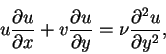
We consider a two-dimensional jet as illustrated in the figure below. x is the horizontal coordinate and y is the vertical coordinate. u and v are, respectively, the horizontal and vertical fluid velocities. The jet in the direction of the x axis generates a flow where the fluid velocity along the y axis tends to zero. We assume that the boundary layer approximation is valid and the governing equation for the fluid motion are equations (2.21) to (2.23), but with
 .
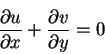
The pressure does not vary in the y direction according to equation (2.22), so the pressure is constant across the boundary layer and its gradient is given by the pressure gradient outside the boundary layer. For this problem there is no pressure gradient, so the governing equations for the fluid motion are
.
The pressure does not vary in the y direction according to equation (2.22), so the pressure is constant across the boundary layer and its gradient is given by the pressure gradient outside the boundary layer. For this problem there is no pressure gradient, so the governing equations for the fluid motion are
 |
(146) |
 |
(147) |
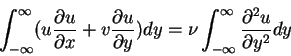
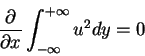
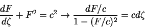
Next, we integrate equation (8.146) with respect to the y variable from  to
to  ,
which gives
,
which gives
 |
(148) |
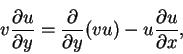
We can write
and if we multiply the continuity equation (8.147) by u, we can write the equation above as
 |
(149) |
Next, we substitute equation (8.149) into equation (8.148), we perform the integration and we use the boundary condition
 |
(150) |
Equation (8.148) simplifies to
 |
(151) |
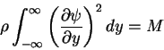
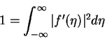
Thus, the momentum flux is constant in x. In other words,
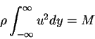 |
(152) |
We call  the order of the magnitude of the boundary layer thickness at position x. Since the orifice is very small we have
 .
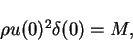
At the orifice the equation (8.152) can be written as
.
At the orifice the equation (8.152) can be written as
 |
(153) |
which implies that
 |
(154) |
The Mass flux at the orifice is
 |
(155) |
hence unimportant. A jet is the result of a momentum source, not a volume source. Next, we are going to solve the boundary layer equations for the jet. We introduce the stream function  related to the velocities u and v according to the equations
 |
(156) |
 |
(157) |
In terms of the stream function, the x momentum equation (8.146) assume the form
 |
(158) |
with the boundary conditions
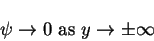 |
(159) |
and
 |
(160) |
We are going to solve the boundary value problem given by equations (8.158) to (8.160) by looking for a similarity solution. We look for a one-parameter transformation of variables y, x and
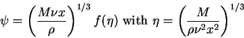
under which the equations of the boundary value problem mentioned above are invariant. A particular useful transformation is
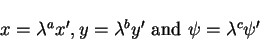 |
(161) |
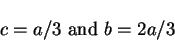
The requirement of invariance of the boundary value problem (8.158) to (8.160) under such transformation implies that
and no information is gained from equation (8.160). From the equations (8.162) and (8.163) we obtain
 |
(164) |
This suggest that we take
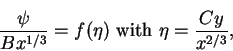 |
(165) |
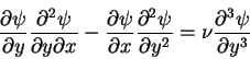
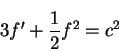
where the coefficients B and C are chosen to simplify the appearance of the final equation. We substitute (8.165) into equation (8.158), which gives the ordinary differential equation
|
3f'''+(f')2+ff'' = 0,
|
(166) |
and for
and  we have
 |
(167) |
the boundary conditions become
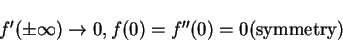 |
(168) |
and
 |
(169) |
Now we integrate equation (8.166) once with respect to ,
which gives
and integrating again
 |
(170) |
We now write
 and
and
 .
then equation (8.170) assumes the form
.
then equation (8.170) assumes the form
 |
(171) |
which can be integrated in closed form, so we have
 |
(172) |
since F(0) = 0. Thus
 |
(173) |
We substitute the equation above for f in the boundary condition (8.169), which gives
 |
(174) |
Finally, we write
 |
(175) |
The final solution has the form
 |
(176) |
and for the velocities we have
 |
(177) |
 |
(178) |
Next, we discuss the implications of the results obtained above. The jet width can be defined by
 such that
 .
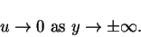
Then from equation (8.177), we realize that the jet width is proportional to x2/3. The centerline velocity, let say umax, according to equation (8.177) is proportional to x-1/3. As
.
Then from equation (8.177), we realize that the jet width is proportional to x2/3. The centerline velocity, let say umax, according to equation (8.177) is proportional to x-1/3. As
 ,
according to equation (8.178),
,
according to equation (8.178),
 .
This implies a that there is entrainment from the jet eddges as show in the figure 4. If we define the Reynolds number as
.
This implies a that there is entrainment from the jet eddges as show in the figure 4. If we define the Reynolds number as
 ,
equation (8.177) implies that
,
equation (8.177) implies that
 .
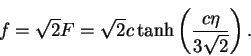
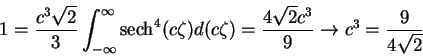
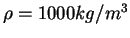
To illustrate the streamlines for the flow generated by the jet, we present figure 3. The velocity field is illustrated in figure 3.
.
To illustrate the streamlines for the flow generated by the jet, we present figure 3. The velocity field is illustrated in figure 3.
Figure:
Streamlines obtained from equation (8.176) with
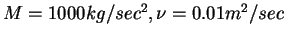 and
and
 .
.
|
|
Figure:
Velocity field obtained from equations (8.177) and (8.178) with
and
.
|
|
Next: About this document ...
Up: No Title
Previous: Stagnation Point flow.
Karl P Burr
2003-03-12
![\includegraphics[width=5.5in,height=5.5in]{ps/psi.eps}](img238.gif)
![\includegraphics[width=5.5in,height=5.5in]{ps/v_field.eps}](img239.gif)