
November 1998
This paper examines the effect of the Kyoto Protocol on developing economies using marginal abatement curves generated by MIT's Emissions Prediction and Policy Assessment model (EPPA). In particular, the paper addresses how developing countries are affected by the scope of CO2 emissions trading, by various limitations that Annex I countries might place on emissions trading, by the nature of the Clean Development Mechanism, and by changes in the international trade flows in conventional goods and services. In general, it is found that developing countries benefit from emissions trading, both from the new export opportunities and by the lesser distortion of Annex I economies. This effect is particularly pronounced for energy exporting countries since Annex I countries are able to substitute cheaper reductions of coal emissions in developing countries for more expensive reductions of oil emissions within Annex I. The paper also highlights the implications of the apparent inelastic demand for tradable permits from non-Annex I countries and the conflict between revenue maximization and other goals assigned to the Clean Development Mechanism.
1. INTRODUCTION
The Kyoto Protocol recognizes a strong linkage between CO2 emission reduction goals, emissions trading, and the role of developing economies. Annex B parties, generally the industrialized nations, have set targets that, for most, imply a significant reduction of CO2-equivalent emissions by 2010. The ability and even willingness of Annex B parties to achieve these targets will depend on the cost of abatement. The cheapest sources of CO2 emission reductions are found, not in the Annex B countries, but in the developing economies (or non-Annex B parties), which for historic and equity reasons are not expected to contribute to the global emissions reduction in the near term. Since the location of CO2 emissions does not matter from a global warming perspective, the achievement of the Kyoto targets will depend in large part upon the ability of Annex B countries to substitute cheaper emission reductions in non-Annex B regions for equivalent abatement at home. In providing a mechanism for this exchange, emissions trading not only reduces the cost of meeting the Kyoto goals for Annex B parties, but also provides a new source of export earnings for non-Annex B parties.
Developing country interest in emissions trading is not limited to the potential for new export earnings. Achieving the goals set at Kyoto will change patterns of consumption and production within Annex B nations; and these changes will have inevitable effects on the flows of internationally traded goods. As a result, developing countries will be affected through conventional trade linkages with the Annex B countries; however, these effects, both favorable and unfavorable, will be diminished to the extent that emissions trading reduces the cost of achieving the Kyoto targets.
In examining the effects of the Kyoto Protocol upon non-Annex B parties, we assume that the Annex B goals are met, and we focus in particular on how emissions trading would affect the developing countries. We refer to emissions trading generically, to include bubbles, joint implementation, allowance or credit systems, and perhaps other forms yet to be devised. The chief practical distinction among these forms concerns the transaction cost involved in effecting an individual trade.
The paper relies heavily upon the use of marginal abatement curves (MACs). These curves represent the marginal cost of reducing carbon emissions by different amounts within an economy. The details of their construction, and the elaboration of the aggregate demand and supply curves for carbon permits which are drawn from them, are explained in Appendix A. The MACs used here are generated using MIT's Emissions Prediction and Policy Assessment (EPPA) model (Yang et al. 1996). This is a multi-sectoral, multi-regional, computable general equilibrium (CGE) model of global economic activity, energy use and carbon emissions. The underlying model simulates real emission reductions, so that our analysis implicitly assumes that the "additionality" criterion established in the Kyoto Protocol [Arts. 6.1(b) and 12.5(c)] is satisfied. We do not attempt to address the considerable political and practical problems of measurement and verification that are associated with this criterion, but we will account for the effect of these problems in a subsequent section. [1]
The main body of the paper consists of five sections. Section 2 uses the MACs to analyze three basic cases: no emissions trading, emissions trading limited to Annex B parties (including the Former Soviet Union), and full global trading. Results are presented in graphical form in the text, and the regional detail--in terms of abatement, costs, emission permit trade and prices for all the cases discussed--is presented in tabular form in Appendix B.
The next three sections address the effects of various departures from the three basic cases. The first departure, in Section 3, is the effect of limitations on imports of emission permits, as might correspond to the "supplementarity" criterion included in the Kyoto Protocol [Arts. 6.1(d) and 17] or to the recent call by the EU environmental ministers for a "concrete ceiling" on emissions trading. Section 4 evaluates the effect of surcharges on emission permits generated under the Clean Development Mechanism (CDM), as also provided in the Kyoto Protocol [Art. 12.8], and of non-competitive pricing. The third departure, discussed in Section 5, is the effect of a smaller supply of permits from the non-Annex B regions than is indicated by EPPA's assumptions of complete economic rationality and zero transaction costs, which we term "inefficient supply."
In Sections 2 through 5, the measure of welfare used is the total direct resource cost required to meet the emissions constraint. As explained in Appendix A, for any country this cost is the area under its marginal abatement curve up to any point of constraint, corrected for any purchase or sale of emissions permits. This is the conventional measure which is generated using the MAC approach. However, because the MACs are generated at the country level, they are not able to take account of effects that are mediated through international trade in energy or other goods. As shown in Appendix A, the MAC results themselves are not sensitive to trade effects. Nevertheless, these effects will influence sub-national details, such as patterns of trade in particular goods and activity at the sectoral level. To explore these effects, we depart from the MAC analysis in Section 6, and present results taken directly from the EPPA model. In Section 7 we offer some concluding observations.
In conducting our analysis, we will make frequent reference to the twelve regions represented in EPPA, which are listed below with the model's acronyms. The CO2 emission reductions required of Annex B regions are calculated as the differences between EPPA's predicted emissions for these regions in 2010 and the goals established at Kyoto for the constituent parties, which are generally stated as a percentage of 1990 emissions, as indicated in Table 1. [2]
Definition of Regions in the EPPA Model
| ANNEX B REGIONS[2] | NON-ANNEX B REGIONS | |
| USA: USA | EEX: Energy Exporting Countries | |
| JPN: Japan | CHN: China | |
| EEC: European Union (EC-12 as of 1992) | IND: India | |
| OOE: Other OECD Countries | DAE: Dynamic Asian Economies | |
| EET: Eastern Europe | BRA: Brazil | |
| FSU: Former Soviet Union | ROW: Rest of World |
Table 1. Emissions Levels Corresponding to Kyoto Commitments
USA
JPN
EEC
OOE
EET
FSU
Non-Annex B
Reference emissions 1990 (Mton)
1362
298
822
318
266
891
2022
Reference emissions 2010 (Mton)
1838
424
1064
472
395
763
4142
Kyoto commitments / 1990
93%
94%
92%
94.5%
104%
98%
NA
Hence Emissions Target in 2010 (Mton)
1267
280
756
301
273
873
4142
i.e. Reduction / ref (Mton)
571
144
308
171
118
0
NA
i.e. Reduction / ref (%)
31%
34%
29%
36%
30%
0
NA
"hot air" (Mton)
0
0
0
0
0
111
NA
Only five of the six EPPA regions encompassing Annex B countries are constrained by the commitment made at Kyoto[3] and these five will subsequently be termed the Kyoto-constrained regions. For the sixth Annex B region, the FSU, emissions are predicted to be below the aggregate level to which the principal nations constituting the FSURussia, the Ukraine, and the Balticscommitted at Kyoto. The difference between the FSU commitment and predicted emissions is controversially called "hot air," but in our analysis we assume that it constitutes a "right to emit" that can be exported. For the non-Annex B regions, as well as for the FSU, any reduction from 2010 reference emissions also generates a permit for export to the Kyoto-constrained regions.
2. THREE BASIC CASES: No Trading, Annex B Trading and Full Global Trading
Three basic cases are used to illustrate the effects of the Kyoto Protocol and the role of emissions trading. The first case is an autarkic one in which Annex B parties meet their Kyoto commitments without any emissions trading. As a result, the FSU and non-Annex B regions are affected only through the prices and quantities of goods traded with the Kyoto-constrained regions. In the second case, Annex B parties (including the FSU) trade emission permits among themselves. Emissions trading within Annex B reduces the costs of the Kyoto commitment for the constrained regions, and the FSU finds a new source of export revenue; but non-Annex B countries will continue to be affected only through conventional trade linkages. The third basic case examines emissions trading on a global scale in which non-Annex B countries join the FSU in earning export revenue from supplying permits to Annex B countries. Further variations of these basic cases will be developed in subsequent sections, but these three frame the salient alternatives.
2.1 The Autarkic, No-Trading Case
Figure 1 presents the MACs and the costs associated with the carbon emission reductions required of each of the Kyoto-constrained regions (excluding the FSU) when there is no emissions trading.[4] The diamond symbols on the MACs indicate, on the horizontal axis, the quantity of abatement required of each region (cf. Table 1), and, on the vertical axis, the shadow price of carbon for the region. The shadow price is the marginal cost for the last ton abated. The autarkic marginal cost of abatement for Japan ($584/ton) is much higher than the marginal costs for the EEC ($273), the OOE ($233), the USA ($186), or the EET ($116). The areas under the curves represent the total costs of abatement for each region, which sum to $120 billion.[5] The details are shown in Appendix B, Table A.
Figure 1. Annex B Regions Meeting their Kyoto Commitment, No Trading. (Table A)
With no emissions trading, there are no export earnings for the FSU or the non-Annex B regions. None of these regions would have any incentive to abate in order to generate "rights to emit" for export; and, of course, the FSU would not be able to export its "hot air."
2.2 Annex B Trading
Figure 2 shows the effect of Annex B trading on the Kyoto-constrained regions. At the market clearing price of $127/ton, the OECD regions (USA, EEC, JPN, OOE) are importers of permits and the EET and FSU are exporters. As an unconstrained Annex B party, the FSU accounts for virtually all of the exports (98%). As shown in Figure 3, about a third of these consist of "hot air," with a cost of zero; but the remaining exports are generated by abatement undertaken to earn additional export profits up to the point where marginal abatement cost equals the market price. It costs the FSU $10 billion to abate 234 megatons (Mton), but the permits can be sold for $30 billion for a net gain of $20 billion. When added to the $14 billion earned for exporting 111 Mton of the unused Kyoto entitlement, the FSU's total gain from emissions trading is $34 billion.
Figure 2. Annex B Meeting their Kyoto Commitment, No Trading/Trading. (Table B)
For the five Kyoto-constrained regions depicted on Figure 2, the cost of meeting the Kyoto commitment is reduced by $32 billion. This is the area of the hatched triangles, which represent costly domestic abatement avoided by importing permits for the four OECD regions and the export earnings for the EET. From the standpoint of world resource use, the aggregate cost of meeting the Kyoto commitments is much lower with Annex B trade ($54 billion) than without ($120 billion). The total gains from emissions trading are$66 billion, split about evenly between the FSU ($34 billion) and the OECD + EET ($32 billion).
Figure 3. Trade with FSU: The "Hot Air" Effect.
The distribution of the reduction in costs (that is, the gains from emissions trading for the Kyoto-constrained regions) is distributed roughly in proportion to autarkic marginal cost. The two regions with the highest autarkic marginal costs, Japan and the EEC, benefit the most from traded permits. Japan imports 66% of its reduction requirement and reduces its cost by $19 billion. The EEC imports 35% of its reduction requirement and reduces its cost by $7 billion. These two regions account for about one-third of the total emission reduction requirement for the five Kyoto-constrained regions, and about five-sixths of the gains from emissions trading for these regions accrue to them. The other three regions are characterized by autarkic marginal costs much closer to the Annex B market price; consequently, they trade much less. The USA and OOE are importers for 19% and 25% of their respective requirements, and the EET reduces emissions by 5% more than required in order to export permits. The gains for these regions, which account for two-thirds of the total reduction requirement, total $5 billion, about a sixth of the gains from trading for the Kyoto-constrained regions.
This distribution of the gains from trade reflects an important feature of emissions trading. Regions with autarkic marginal cost farther from the trading equilibrium will import or export more (and benefit more) than those regions with autarkic marginal cost closer to the trading equilibrium. Thus, Japan and the EEC benefit most from emissions trading among the importers, as does the FSU, not just because of the "hot air," but also because its autarkic marginal cost ($0/ton) is far from the market price.
2.3 Full Global Trading
To illustrate full global trading, we rely on aggregate supply and demand curves for emissions permits (not abatement), as explained in the Appendix A and illustrated in Figure 4. These curves indicate the total quantities of permits that would be supplied or demanded at various price levels in a given market. In Figure 4, there is only one demand curve because the Kyoto-constrained regions are the same in both the Annex B and the global markets. Only the supply changes, reflecting the large amount of low-cost carbon abatement that becomes potentially available with the shift to global trading. The ample supply of permits from non-Annex B regions results in a market price that is much lower ($24/ton) than in the Annex B trading case. The total cost of reducing global CO2 emissions to achieve the Kyoto goals is reduced dramatically: $11 billion vs. $54 billion or $120 billion in the other two cases!

Figure 4. Aggregated Supply and Demand Curves for 2010 under Kyoto Constraints. Annex B Trading / World Trading. (Table C)
At this price, the Kyoto-constrained regions depend far more on imports than when trading was restricted to Annex B regions only. In the aggregate, 71% of OECD + EET commitments are met by importing emission permits from non-constrained regions; and the percentage reliance upon imports reflects autarkic marginal cost: Japan, 92%; EEC, 76%; USA, 68%; OOE, 66% and EET, 56%. On the suppliers' side, three countries account for the bulk of exports: China (47%), the FSU (23%) and India (11%), hence 81% altogether. Whether because of relatively small size or high relative abatement costs, the remaining four non-Annex B regions are small suppliers of emission permits to the Annex B regions.
With full global trading, the gains from emissions trading are much greater for the Kyoto-constrained regions ($94 billion vs. $32 billionwith Annex B trading). The non-Annex B regions gain $10 billion by exporting permits, but their gains are markedly less than those of the Kyoto-constrained regions. The FSU is the only party that is made worse off by this widening of the market. At $24/ton, the FSU abates about half as much as before, (101 Mton), and the "hot air" is worth much less. As a result, the FSU's net gain ($4 billion) in the global market is much less than its $34 billion gain when it does not compete with the non-Annex B regions.
The distribution of the gains from emissions trading in the global market illustrates again the feature of emissions trading we just noted: regions whose autarkic marginal cost is further from the equilibrium price benefit more than regions whose marginal cost is closer to that price. In this global trading case, the clearing price is much closer to the suppliers' autarkic marginal cost ($0/ton) than it is to the autarkic marginal cost of any of the importers.
2.4 Effect of Higher and Lower Economic Growth
The three basic cases, and those to be presented hereafter, provide point estimates of prices, quantities and costs. In this section, we briefly note the effect of different assumptions about economic growth, namely, that it is 10% higher and 10% lower than in the reference EPPA projection for all regions. Figure 5 shows the effect of higher and lower growth rates for illustrative Kyoto-constrained regions (JPN, EEC and USA), and Figure 6shows the effects on aggregate supply and demand for permits in the Annex B and full global markets.
Figure 5. Effect of Lower and Higher Growth Rates (+/- 10%) on the Kyoto Commitment for JPN, EEC, USA. (Tables A' to C')
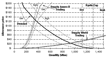
Figure 6. World Supply and Demand in 2010 under Kyoto Constraints. Annex B Trading / World Trading -- Low and High Scenarios. (Tables A'' to C'')
The effects of higher or lower growth on emissions is typically fairly small, always less than 5%, but the Kyoto commitment is fixed so that the effect on the required reduction is amplified. For instance, for the Kyoto-constrained regions, the variation in total required emission is 13 to 14%. Finally, the change in total costs, without trading, is even greater (31-36%), because the most expensive abatement, that on the margin, represented by the hatched area in Figure 5, is what is being increased or decreased by the variation in economic growth.
When aggregated into demand and supply curves for permits, the variation in economic growth has a large effect on demand, but not much on supply since most of the supply comes from unconstrained regions, the FSU or the non-Annex B countries. The chief effect upon supply within the relevant price range is through the influence on hot air. Higher growth reduces hot air and shifts the supply curve inward; and conversely, for lower economic growth.
The effect of higher or lower economic growth on the price and quantities of traded permits is very different in the Annex B and full global trading markets. In the former, the volumes traded change very slightly (12 Mton), but the price varies greatly ($40). In a market limited to Annex B regions, most of the incremental effort required by higher or lower growth translates into more or less domestic abatement. In contrast, for full global trading, the aggregate supply curve is flatter, so that the variation in the volume of traded permits is greater (120 Mton) but the variation in price much less ($6).
The variation in total cost for the Kyoto-constrained regions is slightly greater in the trading cases than in the non-trading case ( 36-42% vs. 31-36%) because with lower or higher growth, greater or smaller amounts of hot air from the FSU enter the trading system.
2.5 Per Capita Emissions
As a further summary statistic, the effect of the Kyoto commitment and of the scope of trading can be shown in per capita terms. Table 2 provides full regional detail, but the essential features can be grasped by reference to Figure 7, where per capita emissions in 2010 are shown for the USA, the five Kyoto-constrained regions as a group, the FSU, the non-Annex B regions, and the world.
The Kyoto commitment reduces per capita emissions in all the Kyoto-constrained regions; however, the reduction is less severe, the greater the scope of trading. In full global trading, as an example, per capita emissions are reduced by 14% on a global scale, but by a greater percentage in the non-Annex B regions since the share of the global emission reduction in the non-Annex B regions is greater than their share of emissions: the aggregate OECD+EET reduction is 9%, while the FSU reduction is 13% and the non-Annex B reduction is 18%.
Table 2. Per Capita Emissions in the Reference Case and in the Three Basic Trading Cases
| USA | JPN | EEC | OOE | EET | OECD + EET | FSU | Non-An. B | World | |
| Population in 2010 (million) | 277.2 | 125.0 | 341.9 | 135.8 | 128.5 | 1008.3 | 324.5 | 5585.7 | 6918.5 |
| Reference (tonC/cap) | 6.63 | 3.39 | 3.11 | 3.48 | 3.07 | 4.16 | 2.35 | 0.74 | 1.32 |
| No Trading (tonC/cap) | 4.57 | 2.24 | 2.21 | 2.21 | 2.15 | 2.86 | 2.35 | 0.74 | 1.13 |
| Annex B Trading (tonC/cap) | 4.95 | 3.00 | 2.52 | 2.53 | 2.11 | 3.20 | 1.63 | 0.74 | 1.14 |
| World Trading (tonC/cap) | 5.98 | 3.30 | 2.90 | 3.04 | 2.67 | 2.78 | 2.04 | 0.61 | 1.14 |
Table 2b.
| EEX | CHN | IND | DAE | BRA | ROW | |
| Population in 2010 (million) | 1103.8 | 1376.9 | 1132.4 | 236.8 | 199.9 | 1535.8 |
| Reference (tonC/cap) | 0.84 | 1.30 | 0.43 | 1.30 | 0.49 | 0.35 |
| World Trading (tonC/cap) | 0.79 | 0.98 | 0.34 | 1.13 | 0.47 | 0.29 |
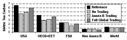
Figure 7. Per Capita Carbon Emissions.
Within the Kyoto-constrained regions, the reduction in per capita emissions varies considerably depending on the extent to which the region imports permits. At one extreme is Japan, where per capita emissions would be less by only 2.7% because it imports 92% of its emission reduction obligation. The greater percentage reductions in the other constrained regions reflect their lesser dependence on permit imports: EEC, -6.7%; USA, -9.8%; OOE, -12.6%; and EET, -13.0%.
Finally, as shown in Fig. 7, neither the Kyoto commitments nor the scope of trading do much to change the ratio of emissions per capita between the industrialized and developing economies of the world.
3. IMPORT LIMITATIONS
The three illustrative cases presented above are based on several
assumptions:
Such assumptions simplify exposition and the analysis of emissions trading, but they are not necessarily realistic. One of the possible departures from this theoretical ideal is a limit on the extent to which an Annex B party can rely on emission permits to reduce what otherwise would be its domestic abatement requirement. The "supplementarity" provisions of the Kyoto Protocol suggest such a limit, although no specific number has been agreed upon. More recently, the EU environmental ministers have called for a "concrete ceiling" on permit imports.
To illustrate the implications of such a restriction, we consider limits of 75%, 50% and 25% on any Annex B party's ability to meet its emission reduction requirement through imported permits.[6] From the full global trading case without restrictions, we know that Japan would optimally realize 92% of its Kyoto commitment through imports, so that with a 75% limit, it would have to abate more domestically. The EEC would also be affected, but to a very slight extent since it would otherwise import 76% of its emission reduction requirement; but none of the other importing regions would be affected. With a 50% limit, all regions would be limited and forced to abate more domestically at higher cost; and at a 25% limit, the reliance on higher cost domestic abatement would be even greater.
Figure 8 shows how the demand curve is shifted inward by such limitations, and Table 3 summarizes the effects on prices (in 1985 US$), quantities and costs. The "No Limit" case is the same as full global trading, and it is provided for comparison.
The effect of import limits upon the exporting regions is predictable. With less demand, the market price falls, fewer "rights to emit" are produced and exported, and there is a drop in the gains to exporters. The effects on importers are twofold. Importers that are not affected by the limitation import more, and at a cheaper price; thus they realize more savings. They are better off because the limitation removes some of the demand by higher cost abaters from the market. Importers who are affected by the limitation also benefit from this lower market price on their imports, but they also incur higher domestic abatement cost.[7] For instance, with the 75% limit, the net balance between these two opposing effects is positive for the EEC (+1.14% gains) but negative for Japan (-1.94%).
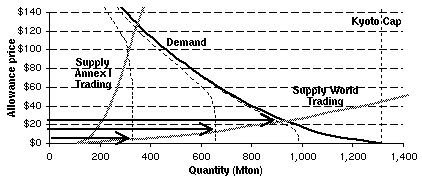
Figure 8. World Supply and Demand in 2010 under Kyoto Constraints. Limitations on Demand: 75%, 50%, and 25%. (Tables D, E, F)
Table 3. Effects of Import Limits on Global Emissions Trading
| No Limit | 75% Limit | 50% Limit | 25% Limit | |
| Market Price (1985 US$/tonC) | $24 | $23 | $13 | $3 |
| Quantity Traded (Mton C) | 935 | 913 | 656 | 328 |
| FSU (Mton) | 211 | 209 | 183 | 148 |
| Non-Annex B (Mton) | 723 | 704 | 473 | 180 |
| World Cost (billion 1985 US$) | $11.2 | $11.9 | $21.7 | $55.3 |
| OECD+EET Cost | $25.6 | $25.4 | $27.1 | $56.1 |
| FSU Gain | $4.2 | $4.0 | $2.0 | $0.5 |
| Non-Annex B Gain | $10.2 | $9.5 | $3.4 | $0.3 |
The overall effect of the 75% limit is relatively slight: the world cost increases slightly (6.5%), the quantity traded is 2% less, the price falls by 4.1%, and the cost to the Kyoto-constrained regions is reduced slightly. With a 50% or 25% limit on imported permits, all the importing regions are restricted, and the price of imports is much lower, $13 and $3, respectively. Among the importing regions, the effects of this tighter limit depend upon the balance between higher domestic abatement costs and cheaper import costs. At 50%, this balance is now negative for both EEC and Japan, but the benefit of the much cheaper imports continues to outweigh the higher domestic abatement costs for the other three importing regions. With a 25% limit, all the importing regions are worse off than they would be without any limit on imports, and the percentage increases in cost are greatest for the higher cost producers of abatement among the importing regions (JPN, +425%; EEC, +123%; OOE, +73%; USA, +58%; EET, +5%).
From the standpoint of the suppliers, the effect of a limitation on imports is to skew the distribution of gains from trading even more heavily in favor of the importing regions. It can be seen in Table 2 that, as the limit becomes more stringent, greater domestic abatement by the importing regions causes world costs to rise, but at least up to the 50% limit, the total cost for the importing regions remains relatively constant, at $25-27 billion. In contrast, for the exporting regions, the gains from emissions trading diminish markedly. The global efficiency losses due to the import limit are effectively shifted to the exporting regions through the lower price of imported permits. Only when the limit becomes very tight and the price of permits is very low, for instance within 25% limit, do the increases in domestic abatement costs outweigh the benefits of cheaper imports, and the importing regions start to absorb the efficiency losses.
The effect of a quantitative limit on imports can be summarized quickly. To the extent that it is binding, it redistributes the gains from trading among the importing regions from those facing the highest abatement costs to those facing the lowest costs. Furthermore, and at least initially, it shifts the increase in global cost caused by a binding import limit onto the suppliers.
4. CDM "SURCHARGES" AND CARTELIZATION OF SUPPLY
Departures from the theoretical ideal can also arise on the supply side. The Kyoto Protocol provides for a Clean Development Mechanism (CDM) by which non-Annex B emissions reductions would be certified and made available as emission permits for Annex B countries. The exact role of the CDM has yet to be defined, but the Protocol does provide that the CDM would apply a surcharge to cover its administrative expense and to collect funds to assist countries "to meet the cost of adaptation" (Article 12.8). Also, because of the inelasticity of demand at low market prices, there is a possibility that suppliers could increase their gains significantly by colluding to limit supply, instead of competing among themselves.
4.1 CDM Surcharges
CDM surcharges would create a wedge between the price paid by consumers and that received by producers, as illustrated in Figure 9 for surcharges of 25%, 50% and 100% of the marginal cost of supply. Table 4provides details concerning prices, quantities and gains. Surcharges of 50% or 100% are beyond any level being discussed currently, but they do illustrate the effects of inelastic demand. Since FSU exports would not be surcharged, we treat the FSU as a competitive supplier in all these cases.
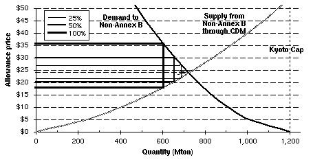
Figure 9. CDM Surcharges: 25%, 50% and 100%. (Tables G, H, I)
Table 4. Prices, Flows and Gains with a CDM Surcharge
| Level of Cdm Surcharge | None | 25% | 50% | 100% |
| Market Price (1985 US$) | $23.8 | $27.4 | $30.6 | $35.9 |
| Producers Marginal Cost (`85$) | $23.8 | $22.0 | $20.4 | $17.9 |
| CDM Net profit (billion $) | $10.2 | $12.6 | $14.4 | $17.0 |
| Profit to producers | $10.2 | $8.9 | $7.9 | $6.3 |
| Surcharge Proceeds | $0 | $3.7 | $6.6 | $10.7 |
| CDM Exports (MtonC) | 723 | 687 | 654 | 602 |
| FSU Exports (MtonC) | 211 | 219 | 225 | 235 |
| FSU Gains (billion $) | $4.2 | $5.0 | $5.7 | $6.9 |
| OECD+EET Cost (billion $) | $25.6 | $28.9 | $31.7 | $36.3 |
| World Cost (billion $) | $11.2 | $15.0 | $18.2 | $23.0 |
The most notable feature of Table 4 is that CDM net profit, defined as revenue minus abatement cost, increases as the surcharge is raised even though importers reduce demand in response to the higher prices. This phenomenon reflects the price inelasticity of demand over this portion of the aggregate demand curve. As would be true of any tax, there is a welfare loss, equal to the increase in world cost as a result of the more expensive abatement undertaken by importers.
The second notable feature of Table 4 is that producer profit decreases on the assumption that surcharge revenue goes to the CDM. Of course, the distribution of the proceeds raised by the surcharge would be a matter for the producers to decide. With inelastic demand, it would be theoretically possible to devise distributions that would keep producers whole and still make funds available for other purposes such as adaptation. Nevertheless, any redistribution of funds for such purposes will reduce what the non-Annex B producers might otherwise receive.
The implicit conflict between producer interests and re-distributive goals has larger implications for the evolution of the global climate regime. It will be readily evident to all non-Annex B producers that the greatest beneficiary from CDM surcharges is the FSU. As a competitive supplier, the FSU benefits directly from the increase of the market price and the increase of its exports. It is able to benefit doubly because, having accepted an Annex B limit on emissions, its exports are not surcharged. The example will be compelling for many non-Annex B producers, who will come to see Annex B accession as a way to by-pass the CDM. Proponents of the CDM will not be pleased, but such action is essential both to the creation of a more efficient global trading system and to achieving the stabilization of atmospheric concentrations of GHGs.[8]
Accession logically implies a transitional role for the CDM. So long as the CDM provides an essential service--recordation, certification and verification--for converting non-Annex B emission reductions into tradable emission permits, a reasonable fee can be charged. But that service, and the attendant role for the CDM, would no longer be needed as non-Annex B parties accept limits and arrange for their own certification and verification as part of the global emissions trading regime.
4.2 Cartelization of Supply
The ability to raise surcharges without diminishing net profit to non-Annex B producers may inspire thoughts of a cartel, not so much because of the CDM, which might serve as a coordinating mechanism, but because of the inelasticity of demand that characterizes the global emissions market.[9] This potential is explored in Table 5, which compares the effects, under full global trading, for a fully competitive market and two alternative assumptions about non-competitive behavior:
1) A CDM cartel in which the FSU is a competitive supplier, and
2) A full supplier monopoly in which the FSU and the non-Annex B countries cooperate through the CDM or an alternative mechanism.
In calculating the gains for the FSU and the non-Annex B regions, we assume that the monopoly rent, the difference between market price and marginal cost, is shared in proportion to the quantity of abatement provided at marginal cost. In doing so, we also assume a highly efficient cartel in which only the lowest cost sources of permits are produced (including the FSU's hot air).
Table 5. Effect of Non-Competitive Behavior on Gains from Trade, Costs and Prices (Tables J to L)
| Competitive case |
Non-Annex B cartel |
Non-Annex B + FSU monopoly | |
| Market Price ($/metric ton C) | $23.8 | $62.7 | $108.2 |
| World Cost (billion 1985US$) | $11.2 | $20.0 | $32.2 |
| Non-Annex B Gains (billion $) | $10.2 | $22.4 | $30.1 |
| FSU Gains (billion $) | $4.2 | $13.8 | $17.4 |
| OECD+EET Gains (billion $) | $94.2 | $63.6 | $39.2 |
Successful monopolization has the expected effects: the market price is higher, as is world resource cost, and the gains from trade are shifted substantially to the suppliers. In the case of the CDM cartel for example, the importing regions lose $32 billion: the $9 billion increase in global costs plus a $23 billion transfer of income to the suppliers. With the full supply monopoly, the importing regions lose another $25 billion, $12 billion in increased resource cost and another $13 billion transfer to the suppliers. Even though this is a dramatic change in the distribution of the gains from permit trade, the Kyoto-constrained regions are still better off (by $7 billion) than if there were no supply at all from the non-Annex B regions. The FSU is, however, always worse off, even when the suppliers successfully create an efficient monopoly.
The incentive to collude would be even greater if limits were placed simultaneously on import demands, since the effect of such limits is to make demand more inelastic. Table 6 makes the point. It shows the effect of the full monopoly on price, world cost and gains when there is no limit on permit imports and when a 50% limit is set.
Table 6. Effect of Monopoly on Gains for Suppliers when Limit on Permit Imports (Tables J to L)
| Limit on imports |
Competitive case |
Non-Annex B + FSU monopoly |
|
| Market Price ($/metric ton C) | No limit | $23.8 | $108.2 |
| 50% limit | $12.5 | $103.4 | |
| World Cost (billion 1985US$) | No limit | $11.2 | $32.2 |
| 50% limit | $21.7 | $37.6 | |
| Non-Annex B Gains (billion $) | No limit | $10.2 | $30.1 |
| 50% limit | $3.4 | $26.2 | |
| FSU Gains (billion $) | No limit | $4.2 | $17.4 |
| 50% limit | $2.0 | $16.3 | |
| OECD + EET Savings (billion $) | No limit | $94.2 | $39.2 |
| 50% limit | $92.6 | $39.8 |
The effect of successful monopoly is much the same whether or not there are import limits. The market price rises to about the same level, $103 vs. $108, world cost increases, and the exporting regions gain significantly at the expense of the importing regions. The effect of a 50% import limit is also much the same whether a competitive market or a monopoly is assumed. The market price is reduced, world cost increases, and producer gains are diminished, but by less when there is a monopoly.
5. INEFFICIENT SUPPLY
Full global trading is an appealing prospect, to importers for the great reductions in cost and to exporters for the possibilities of non-competitive pricing, but both importers and exporters should remember that the potential trading gains shown by CGE models assume complete economic rationality and negligible transactions cost.[10] The more likely contour of global emissions trading is that this potential will not spring forth full blown once trading is allowed, but that it will develop only slowly as experience is gained. Figure 10 depicts several possibilities for less than fully efficient supply in which it is assumed that 5%, 10%, 15%, 25%, and 50% of the supplies from the FSU and non-Annex B regions are available at every price.[11] The lowest line, corresponding to 100%, is fully efficient global trading.
Figure 10. World Permit Supply and Demand in 2010 under Kyoto Constraints. Limitation on Supply: Suppy = 50%, 25%, 15%, 10%, and 5% of Total. (Tables M to Y)
Inefficient supply could result from several causes. The most serious and most likely is the influence of transaction cost, particularly that involved in meeting the "additionality" criterion. Past experience with credit-based emissions trading systems applied to other environmental problems and with Joint Implementation pilot projects has shown these costs to be large and the quantities traded to be small.[12] Alternatively, a general failure to take full advantage of economic
opportunities presented by emissions trading would also limit the amount of credits available from the non-Annex B regions and the FSU. Finally, some non-Annex B countries have expressed considerable antipathy to emissions trading as a concept; and they may decide not to participate in an emissions trading regime, whether through the CDM or otherwise, for political reasons. It is not possible to assess beforehand to what extent these causes might operate in a global market, but they will certainly be present.
If the supplies from the global market are very small initially, say 5% of the full global potential, then the market price for permits would be relatively high ($181) and the quantities traded small (170 Mton). As experience is gained and supplies become more ample, the quantities traded would increase and prices fall. The gains from emissions trading increase with improved efficiency of supply and they become quite large well before attaining 100% efficiency. As shown in Figure 11, total gains increase steadily, but those for exporters increase only up to a point a little above15%. Thereafter, the relatively inelastic demand causes the gains to exporters to decline, while those to the importers increase dramatically.
Figure 11. Gains from More Efficient Global Trading. (Tables M to Y)
When supply is very inefficient, the market distortions considered earlier have little effect. For example, as severe a limitation on demand as a 25% ceiling would affect only Japan if supplies from the FSU and non-Annex B regions were only 5% of the full potential. And at the prices reflecting very inefficient supply, there would be no gain to monopoly. Nevertheless, as supply becomes more efficient and prices decrease, a limitation on imports would become more binding; and as the market clearing price moved into the inelastic range (below about $110), non-competitive pricing could become more of a concern.
With inefficient supply, the effect of CDM surcharges will also depend on the elasticity of demand. In the inelastic range (low price, large quantity), corresponding to greater supply from the non-Annex B regions, the surcharge can result in greater gains for exporters, so that it is at least possible to keep producers whole (compared to no surcharge) and generate funds for other purposes. However, in the inelastic range (high price, small quantity), any surcharge will reduce the total gain to be shared between producers and other claimants.
As would be expected, inefficient supply implies a higher market price, greater world cost and fewer gains from trade, but the gains will still be substantial and decidedly worth pursuing. The
effects of distortions, such as import limitations and non-competitive pricing, are the same as with fully efficient supply, but the magnitude of the effect is less because there is less to lose. Perhaps the most notable feature of inefficient supply is that the gains to early entrants in the global emissions market will be very large. Thereafter, as is true for any innovator, the large initial reward will dissipate as imitators follow.
6. INTERNATIONAL TRADE IN ENERGY AND NON-ENERGY GOODS
MACs provide a simple and direct way to study emissions trading, but they do not indicate the effect of abatement actions on the prices and quantities of goods in international trade. The effects of emissions reductions may not be restricted to the countries undertaking the abatement actions. Through trade they may be transmitted to countries that made no commitment. In this section, we depart from the use of MACs and examine these other effects using the EPPA results directly.
The central feature driving these trade-in-goods effects is the shadow price for carbon that is faced by the Kyoto-constrained regions, and the effect of that shadow price on the world price for oil and natural gas. Table 7provides a quick summary of those prices for the 2010 reference case and our three basic emissions trading scenarios. Carbon prices are shown in 1985 dollars; oil and gas prices are shown as an index with the 2010 price in the reference case set to 1.0.
Table 7. Carbon And Energy Prices In 2010 For Kyoto-Constrained Regions
| Reference | No Trading | Annex B | Global | |
| Carbon Price | $0 | $116-584 | $127 | $24 |
| Oil Price | 1.0 | 0.90 | 0.95 | 0.99 |
| Natural Gas Price | 1.0 | 0.83 | 0.86 | 0.96 |
Oil and natural gas are treated as Hecksher-Ohlin goods in EPPA, which means that there is complete freedom of trade among regions and a single world price. As a result, restrictions on carbon emissions in Annex B countries lead to lower oil and natural gas prices for producers and consumers throughout the world. In contrast, coal is an Armington good, which means that there is no single world price but a series of regional prices that can be affected by changes in trade flows. Consequently, actions by the Annex B regions will affect coal prices in these regions, but generally not elsewhere, or only through the quantities traded (which are not great.)
As the scope of emissions trading expands and the price of carbon declines, the effect of Kyoto commitments on energy prices diminishes. This effect occurs because one of the cheapest forms of carbon abatement is the reduction of and substitution away from the use of coal. Emissions trading makes it possible to substitute reduced coal use in non-Annex B regions for more expensive abatement that reduces oil and natural gas use in Annex B regions.
The effects on trade patterns of the Kyoto commitments and emissions trading are most usefully observed by comparing the no trading case with full global trading. The former can be viewed as a relatively inefficient way of achieving the goals set at Kyoto, while the latter represents the most efficient way. Emissions trade limited to Annex B is an intermediate case, which we omit because its effects lie between what occurs with no emission trading and with full global trading.[13]
6.1 Trade in Goods with No Emissions Trading
The starting point for the no emissions trading case is the effect of the carbon price on domestic demand in the Kyoto-constrained regions. Table 8 provides the percentage change from the reference prediction for domestic use of sectoral output (production less exports plus imports) by each Kyoto-constrained region. The sectoral breakdown in EPPA includes five energy sectors (oil, gas, coal, electricity and refined oil) and three non-energy sectors (agriculture, energy intensive industries, and other industries).
Table 8. Percent Change in Domestic Use by Sector and Region Due to Kyoto Commitment Without Emissions Trading
| USA | JPN | EEC | OOE | EET | |
| Oil | -3.5% | -19.6% | -4.0% | -7.6% | -3.4% |
| Gas | -11.1% | -24.8% | -10.3% | -14.1% | -12.1% |
| Coal | -54.5% | -48.8% | -52.1% | -63.2% | -49.4% |
| Electricity | -11.1% | -11.3% | -12.2% | -13.1% | -19.7% |
| Refined Oil | -6.5% | -20.3% | -7.7% | -10.6% | -7.7% |
| Agriculture | -0.7% | -2.2% | -0.2% | -0.9% | -0.4% |
| Energy Intensive | -0.5% | -5.1% | -2.6% | -1.7% | -2.2% |
| Other Industries | +0.1% | -1.1% | -0.2% | -0.4% | -0.6% |
With one insignificant exception, all the signs are negative, and they are greatest in magnitude for the energy sectors. Coal is hit hardest with domestic use declining by about half in all regions. However, coal, like electricity and refined oil, is mostly a domestic good so that the international trade effect of this reduction in demand is not particularly great. Oil and gas are more heavily traded internationally, and the effect of the reduction in Annex B demand is a world-wide fall in the price of oil and gas: by 10% and 17%, respectively, as was shown above in Table 6.[14] This reduction in price reduces the income of oil and gas producers throughout the world; and the effect will be particularly large on the two oil and gas exporting regions, the EEX and the FSU. Interestingly, the quantities of oil and gas traded internationally do not change much, but there is a shift in the destination of energy exports away from the Kyoto-constrained regions towards the non-constrained regions, as illustrated next, through trade in energy-intensive goods.
The domestic use of energy-intensive goods declines in all Kyoto-constrained regions; however, the most significant effects show up in the trade balances and domestic output for these goods, as shown in Table 9. The patterns are very clear. The Kyoto-constrained regions reduce production and net exports of energy-intensive goods, while the non-constrained regions increase output and net exports of them. The Kyoto-constrained regions increase imports of these goods, and of the non-taxed carbon that is embodied in them.
Table 9. Changes in Export, Import and Output of Energy Intensive Goods: No Emissions Trading
| Absolute Change in: | USA | JPN | EEC | OOE | EET | FSU | EEX | CHN | IND | DAE | BRA | ROW |
| Net trade | -2.57 | -30.96 | -26.20 | -6.29 | -1.61 | +7.93 | +22.8 | +6.78 | +1.13 | +6.07 | +1.86 | +21.1 |
| Output | -6.90 | -61.68 | -42.25 | -9.31 | -4.99 | +9.81 | +21.1 | +15.3 | +2.74 | +15.8 | +3.46 | +22.9 |
6.2 Comparing the No-Trading Case with Full Global Trading
Meeting the Kyoto commitments with full global trading has much less effect on Annex B demand for oil and gas and on the trade in energy-intensive goods than was the case with no emissions trading, as shown in Table 10and Table 11.
Table 10. Percent Change In Domestic Use By Sector And Region Due to Kyoto Commitment With Full Global Trading
| USA | JPN | EEC | OOE | EET | |
| Oil | -0.2% | -0.2% | -0.2% | -0.3% | -0.5% |
| Gas | -0.5% | -0.5% | -0.7% | -0.04% | -0.9% |
| Coal | -21.5% | -5.0% | -13.2% | -25.0% | -15.4% |
| Electricity | -2.5% | -0.3% | -1.6% | -2.3% | -5.0% |
| Refined Oil | -1.0% | -0.8% | -0.6% | -1.2% | -1.5% |
| Agriculture | -0.1% | -0.1% | -0.03% | -0.1% | +0.2% |
| Energy Intensive | -0.1% | -0.1% | -0.1% | -0.1% | +0.02% |
| Other Industries | -0.1% | -0.1% | -0.1% | -0.1% | -0.1% |
Table 11. Changes In Export, Import And Output Of Energy Intensive Goods: Full Global Trading
| Absolute Change in: |
USA | JPN | EEC | OOE | EET | FSU | EEX | CHN | IND | DAE | BRA | ROW |
| Net trade | +0.37 | +0.30 | -0.09 | +0.16 | +0.19 | -0.71 | +1.61 | -2.60 | -0.94 | +0.53 | -0.02 | +1.22 |
| Output | -0.59 | -0.18 | -0.93 | -0.02 | +0.21 | -1.81 | +0.45 | -8.90 | -2.25 | +0.10 | -0.01 | +1.24 |
The effects of the Kyoto Protocol remain negative, but the magnitudes are much attenuated. Coal use is reduced by at most a quarter; and the effect on other goods is generally less than 1%. The world prices for oil and natural gas are reduced by only 1.3% and 3.5%, respectively, instead of 10% and 17% in the no trading case.
The changes in trade and output of energy-intensive goods are all relatively small; and there is no consistent pattern as in Table 9, because the price of carbon is the same in all countries. Output and the net trade position is most adversely affected in China, India and FSU because their production of energy intensive goods is more dependent on coal, which is the fuel most strongly affected by any positive price on carbon emissions.
6.3 Summary
The effects of the Kyoto Protocol and of emissions trading on non-Annex B regions consist of three analytically separate elements, which can be summarized by the simple matrix in Table 12.
Table 12. Effect of Kyoto and Emissions Trading
| KYOTO EFFECT | No Emissions Trading | Global Emissions Trading |
| Permit Revenues | 0 | + |
| Oil & Gas Export Revenue | - - | - |
| Energy Intensive Goods Trade | + | 0 |
Whether there is emissions trading or not, the effect of the Kyoto commitments on non-Annex B countries is mixed. Without emissions trading, there will be no permit exports, but an increase in the production and export of energy intensive goods can be expected, assuming no protective trade measures are enacted by the Kyoto-constrained regions. With global emissions trading, there will be permit export revenues, but no significant increase in production and exports of energy intensive goods. The revenues of non-Annex B regions that export oil and gas will be adversely affected in either case, but much less so with the lower carbon price associated with a broadened market for emissions permits. In effect, oil and gas exporters benefit as emissions trading makes it possible for Kyoto-constrained regions to substitute reduced coal use in non-Annex B regions for reduced oil and natural gas use at home.
7. CONCLUDING OBSERVATIONS
The effect on developing countries of Annex B actions to comply with the Kyoto Protocol will depend on the particular country and on the success of emissions trading. All developing economies will have an interest in emissions trading as a source of new export earnings, but their interest will extend beyond this new commercial possibility. In particular, oil and gas exporters will have a strong interest in emissions trading as a means to reduce the cost for Annex B parties generally, and specifically to allow Annex B parties to substitute reduced coal emissions abroad for reduced oil and gas emissions at home. It is possible that some countries and sectors would be adversely affected by emissions trading. For instance, the advantage enjoyed by producers of energy-intensive goods will be greater with no emissions trading, assuming that importing embodied carbon is permitted by the Annex B regions. The net balance will be different for various countries, but in general it seems likely that developing countries will benefit from emissions trading.
The gains from emissions trading are potentially very large, fully sufficient to give potential buyers and sellers an economic incentive to support such a system. Most studies of permit trade suggest ample supplies would be offered by non-Annex B regions, at commensurately low prices, yielding large cost reductions for the Kyoto-constrained regions and substantial benefits to non-Annex B regions. The actual supply is likely to be somewhat less, at least initially, due to transactions cost and less than complete participation in the market by non-Annex B regions. Nevertheless, whatever the initial extent of the market and its subsequent development, both importing and exporting parties will gain.
As in any market, the potential for welfare-damaging distortions is always present. Given the undefined meaning of "supplemental" in the Kyoto Protocol, a particularly alarming distortion from the developing country standpoint is a limitation on Annex B imports of emission permits. Not only will such limits depress permit prices and the export earnings of non-Annex B parties, but they will have perverse effects on importing countries. Annex B parties with relatively high domestic abatement costs, and thus higher imports, would be penalized, while those with relatively low domestic abatement costs, and fewer imports, would find the cost of meeting their Kyoto commitments reduced.
The ability of the CDM to impose surcharges to help countries meet the costs of adaptation will depend upon the elasticity of demand, which depends in turn on the supply available from non-Annex B regions. The greater the supply and the lower the price, the greater the ability to impose surcharges without fear of losing revenue. Still, there is an unavoidable conflict between the interests of the producers of the permits and redistributive goals, since whatever is redistributed could as well be kept by the producers.
The FSU and the non-Annex B countries appear as clear rivals to each other in the stylized cases we have presented, but casting this rivalry in geopolitical terms obscures a more practical aspect. Neither the Annex B nor the global market will spring into life full blown as soon as the appropriate institutional arrangements are made; instead these markets will develop slowly over time. The stylized Annex B market should be thought of as illustrating the potential gains for first entrants of whatever provenance into a new and expanding market. Those gains will inevitably be dissipated as others follow, so that the conflict, which appears here as one between the FSU and non-Annex B regions, is really one between the early entrants and later followers.
The FSU does however have one large advantage. Assuming effective accounting and enforcement, its acceptance of an Annex B emission limitation removes the high costs of establishing additionality, which will be required of projects in non-Annex B countries. This example will encourage the most enterprising non-Annex B countries to accede to Annex B to capture more of the large gains of early emissions trading. In doing so, these parties will foster more efficient emissions trading and promote the ultimate goals of the Kyoto Protocol, but they will also necessarily reduce the ability of the CDM to act as a re-distributive mechanism.
8. ACKNOWLEGMENTS
Funding for this paper from the World Bank is gratefully acknowledged. We are also very much indebted to Ian Sue Wing for modeling support and to the following individuals for comment on earlier versions of the paper: at MIT, Richard Eckaus, David Reiner and Mustafa Babiker; and at the World Bank, Zmarak Shalizi, Ken Chomitz and Maureen Cropper.
9. REFERENCES
Ellerman, A.D. and A. Decaux, 1998, Analysis of Post-Kyoto Emissions Trading Using Marginal Abatement Curves, MIT Joint Program on the Science and Policy of Global Change Report No. 40, October, Cambridge, MA.
Jacoby, H.D., R.G. Prinn and R. Schmalensee, 1998, Kyoto's Unfinished Business, Foreign Affairs, 77(4):54-66, July/August.
Prinn, R.G., et al., 1998, Integrated Global System Model: Feedbacks and Sensitivity Studies, Climatic Change, forthcoming; MIT Joint Program on the Science and Policy of Global Change Report No. 36, May, Cambridge, MA.
United Nations Conference on Trade and Development (UNCTAD), 1998, Greenhouse Gas Emissions Trading: Defining the Principles, Modalities, Rules and Guidelines for Verification, Reporting and Accountability, Geneva, Switzerland, draft of July.
United Nations Framework Convention on Climate Change, 1997, Kyoto Protocol.
United States Government, Executive Office of the President, 1998, The Kyoto Protocol and the President's Policies to Address Climate Change: Administration Economic Analysis, July.
Yang, Z., et al., 1996, The MIT Emissions Prediction and Policy Analysis (EPPA) Model, MIT Joint Program on the Science and Policy of Global Change Report No. 6, Cambridge, MA.
Yang, Z. and H.D. Jacoby, 1997, Necessary Conditions for Stabilization Agreements, MIT Joint Program on the Science and Policy of Global Change Report No. 26, Cambridge, MA.
A.1 What are Marginal Abatement Curves and What Do They Represent?
A CGE model will produce a shadow price for any constraint on carbon emissions for a given region R at time T. An example would be a 10% reduction below the reference case for USA in 2010. This price indicates the marginal cost of reducing the last ton of carbon required to meet the constraint. As might be expected in a proper CGE model, the shadow prices corresponding to constraints of increasing severity rise as an increasing function of emissions reduction. A Marginal Abatement Curve is described by generating the plots of the shadow prices corresponding to constraints of increasing severity at time T, then drawing a line joining the plots, as in Figure A1. Each plot on the curve for region R at time T represents the marginal cost (p) of abating an additional unit of carbon emissions at quantity q. The integral under the curve (hatched area) represents the total abatement cost associated with each level of abatement, that is, the resources re-allocated to abatement because of the constraint.
Figure A1. Marginal Abatement Curves
A.2 How Can MACs Be Used for Trade Studies?
If several regions commit to achieve emission reductions at the same time and there is some prediction of what emissions would be without the commitment, the abatement required can be represented as a point on each region's marginal abatement curve. [16] Moreover, if the marginal costs associated with those reductions are different across regions, the aggregate cost of meeting the commitments will be less to the extent that a region with higher marginal costs can induce a region with lower marginal costs to abate more on its behalf. Figure A2 illustrates the gains from trading for two regions, R1 and R2, subject to the constraints: CO2 abated = q1 for R1 and q2 for R2.
Figure A2. Marginal Abatement Curves Used for Trade Studies.
By abating more, the lower cost region produces "rights to emit," or emission permits, which it can sell to the higher cost region which would thereby avoid a like amount of higher cost domestic abatement. Thus, the difference in the marginal costs associated with each region's commitment in the absence of trade creates a potential gain to be shared in some manner between them. The aggregate emission reduction will be achieved at least cost when the two regions trade until their marginal abatement costs are equal at what will then be the market clearing price for the "right to emit" carbon.
Table A1 displays the cost calculations in the no trading and trading cases. These cost calculations can easily be generalized to N regions, and they constitute the basis for emissions trading studies using MACs.
Table A1. Basics of Trade Studies
| No Trade | Trade between R1 and R2 | |
| Constraints | R1: q1 abated R2: q2 abated |
R1 and R2: q1 + q2 abated |
| Marginal Cost / Market Price | R1:
p1 R2: p2 |
R1
and R2: p' such that p'1(q'1) =
p'2(q'2) = p' and q'1 + q'2 = q1 + q2 |
| Abatement Cost | R1:
area AOQ1 R2: area BOQ2 |
R1:
area (A'OQ'1) R2: area (B'OQ'2) |
| Emission Permits Trading | NA | R1:
buys right to emit q1 - q'1 R2: sells right to emit q'2 - q2 = q1 - q'1 |
| Imports (+) / Exports (-) Flows | NA | R1:
pays p' x (q1 - q'1) = area
(A'I1Q1Q'1) to
R2 R2: receives p' x (q'2 - q2) = area (B'I2Q2Q'2) from R1 |
| Total Cost | R1:
area AOQ1 R2: area BOQ2 |
R1:
area (A'OQ'1) + area (A'I1Q1Q'1)
< area (AOQ1) R2: area (B'OQ'2) - area (B'I2Q2Q'2) < area (BOQ2) |
| Savings from Trading | NA | R1:
area (AI1A') (hatched) R2: area (BI2B') (hatched) |
A.3 How are MACs Generated from CGE Models?
The CGE model we use to generate MACs is the MIT Emissions Prediction and Policy Assessment (EEPA) model. It is a multi-sectoral, multi-regional global model of economic activity, energy use and greenhouse gas (GHG) emissions that is part of MIT's larger Integrated Global Systems Model (IGSM).[17] As such, EPPA is frequently used to predict emissions and to assess the costs associated with constraints on carbon emissions. Although EPPA predicts emissions and assesses costs through the year 2100, this study takes the year 2010 as representative of the first commitment period, which includes the years 2008 through 2012. The model keeps track of five vintages of capital. Version 2.6 of the model incorporates two backstop technologies; however, because these energy sources will not play a substantial role in 2010, they are omitted from the calculations presented here.
To build the MACs, we run the EPPA model under different constraints corresponding to different levels of carbon abatement, such as 10%, 20%, or 30% of reference emissions in the year 2010. For each set of constraints, the corresponding, regional shadow prices of carbon are an output of the model (in 1985 US$).[18] The shadow prices for each region can then be plotted as a function of the level of abatement, and a line can be fitted to the plots to get the MAC for that region and time.
As an example, Figure A3 shows the results obtained for the four OECD regions in 2010 when the policies applied are: proportional reductions by all OECD regions (1, 5, 10, 15, 20, 30 and 40% of reference 2010 emissions), and no reduction by other regions. Here, the shadow prices have been plotted as a function of the percentage of carbon emission reduction (and not the absolute quantities), in order to normalize for the size of the regions and to show the variation in relative cost across regions. For any equal percentage reduction among the OECD regions, the abatement of the corresponding quantities would cost most in Japan, then in EEC, and least in USA and OOE.
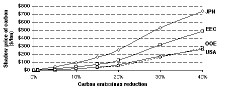
Figure A3. EPPA-Generated Marginal Abetaement Curves for 2010. OECD Regions, Proportional Reductions, No Trading.
Similar curves can be obtained for all regions. For example, the same proportional reductions can be applied to all of EPPA's twelve regions at the same time.[19] Figure A4 displays the marginal abatement curves thus obtained. It shows where it is the cheapest to abate carbon emissions (India and China) and where it is the most expensive (Japan).
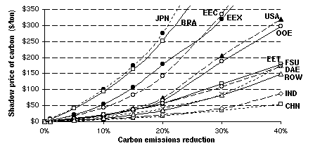
Figure A4. EPPA-Generated Martinal Abatement Curves for 2010. All Regions, Proportional Reductions, No Trading.
Stating marginal cost in terms of the proportional reduction reveals the relative cost of carbon abatement among the twelve EPPA regions, but it does not indicate the importance of various regions in an emissions trading market. For example, as shown in Fig. A4, both China and India are relatively low cost suppliers of abatement. However, as shown in Figure A5, China is a significantly greater potential supplier of abatement than India by the simple fact that its reference emissions are predicted to be 3.5 times as large (1,792 vs. 486 Mton).[20] China is about 70% more carbon intensive than India; and its economy is predicted to be about twice the size of India's in 2010. As a result, for any given price, China supplies a much larger quantity of permits than India. China is by far the largest potential source of emissions permits from the non-Annex B regions.For instance, if the market price for emissions permits were $50, China would provide about 700 Mton of emissions reduction, while the five other regions combined would provide only 400 Mton.
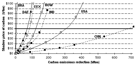
Figure A5. EPPA-Generated Marginal Abatement Curves for 2010. Non-Annex B regions, Proportional Reductions, No Trading.
A.4 Assessing the "Robustness" of MACs with Regard to the Policy Applied
One question that arises immediately from our use of equal proportional reduction across regions to generate the MACs is whether the location of these curves, or more generally, the cost associated with any given level of carbon abatement, is affected by differing levels of abatement in other regions. For instance, as can be seen in Table 1, the levels of implied abatement corresponding to the Kyoto commitment are not strictly proportional, and with emissions trading, we would not expect the percentage reductions among regions to remain the same. Will region R1's MAC look different depending on whether region R2 reduces by 10% or 40%? In a model with international trade in all goods, such as EPPA, there is the possibility that a 40% reduction by region R2 would alter trade flows such that abatement of, say, 100 Mton by R1 would cost more (or less) than if R2 reduced emissions by only 10%. This fundamental question is that of the robustness of the MACs. And indeed, a drawing like Fig. 2 and the simple method we have deduced from it assume this robustness (one curve for each region, whatever the reductions in other regions). The answer: they are robust.
For example, Figure A6 shows simultaneously the two sets of MACs corresponding to varying levels of OECD abatement assuming no emissions trading and fully efficient emissions trading.[21] The curves in both sets are similar (less than 10% variation in price for any given level of abatement), thus showing that the MACs are robust with regard to this change of policy. We have made similar comparisons for Annex B trading and global trading, and we have examined one region's MAC (the USA) when all other regions vary from reference to as much as a 60% reduction. In all cases, we have found the same fundamental result: whatever the trading scheme, whatever the extent of the market, the marginal abatement curves are almost identical. These model results indicate that abatement cost in a region is largely independent of abatement efforts in other regions.
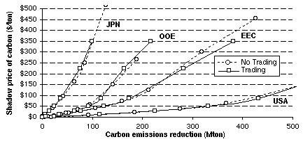
Figure A6. EPPA-Generated Marginal Abatement Curves for 2010. OECD Proportional Reductions, No Trading and OECD Trading.
Our conclusion is that MACs, and more generally, the costs associated with a given level of domestic abatement, are sufficiently insensitive to different levels of abatement among regions and the scope of emissions trading to justify the analytic method applied here.
A.5 Analytical Approximations: A Simple Tool for Trade Studies
Robustness implies that at time T each region has a unique marginal abatement curve. This result allows independent use of marginal abatement curves, once generated from CGE model, and makes trade analysis straightforward. Such an analysis can be even further simplified if each curve is described by a single mathematical expression because, once we have the equations of the MACs, the cost calculations (i.e. integration under the curves) are simple and rapid.
Figure A7 shows, for the OECD regions, that we can fit very simple analytical curves to the sets of plots resulting from the EPPA runs, and that those fits are very good (for each curve, R2 very close to 1.0). This result holds for all the other regions as well. The curves that best fit the EPPA-generated plots are of the form: P = aQ2 + bQ, where Q is the amount of carbon abatement in Mton and P is the marginal cost, or shadow price, of carbon in 1985 US$. By integration, the total cost of abatement is C = 1/3 x aQ3 + 1/2 x bQ2. Table A2 displays the coefficients a and b for each region in 2010, as well as the coefficient of determination R2.
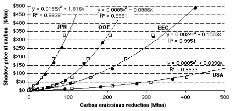
Figure A7. Marginal Abatement Curves for 2010. OECD Regions, Polynomial Approximations.
Table A2. Coefficients of the Approximations of the MACs of the Form: P = aQ2 + bQ
| Region | a | B | R2 | Region | a | b | R2 |
| USA | 0.0005 | 0.0398 | 0.9923 | EEX | 0.0032 | 0.3029 | 0.9983 |
| JPN | 0.0155 | 1.816 | 0.9938 | CHN | 0.00007 | 0.0239 | 0.9992 |
| EEC | 0.0024 | 0.1503 | 0.9951 | IND | 0.0015 | 0.0787 | 0.9970 |
| OOE | 0.0085 | -0.0986 | 0.9981 | DAE | 0.0047 | 0.3774 | 0.9996 |
| EET | 0.0079 | 0.0486 | 0.9973 | BRA | 0.5612 | 8.4974 | 0.9997 |
| FSU | 0.0023 | 0.0042 | 0.9938 | ROW | 0.0021 | 0.0805 | 0.9967 |
In using these approximations, analysts should keep in mind that the price of this simplicity is some loss of the details of the general equilibrium features of the underlying model. The robustness of the curves assures us that the relation between price and quantity of abatement is relatively fixed, but the curves do not capture all the effects of emissions trading. Since the EPPA model remains our primary analysis tool, we have run the model in every policy case we studied in order both to ensure that the approximations are not misleading and to capture any possible side effects. The prices and quantities for abatement were all very close to the approximations, but there is a side effect that the MACs do not show: "leakage." When carbon emissions are constrained for only a sub-set of regions, carbon emissions tend to "leak" to non-constrained regions. Nevertheless, these effects are not essential to the analysis conducted here;[22] and the analytical approximations are a powerful computational shortcut to particular results. They also provide a convenient way to represent graphically the results of the trading analysis.
A.6 Construction of Aggregate Supply and Demand Curves
Marginal abatement curves are the basis for determining the demand and supply for emission permits in any given market. Emission permits represent "rights to emit" and these rights can be produced by some party abating more than it is required to do, or undertaking some abatement when not required to do so. The willingness of any party to produce these permits is illustrated by Figure A8. The vertical dotted line represents the amount of abatement required for a region to meet its Kyoto commitment. In the absence of any emissions trading it would abate the amount indicated by the intersection of this line with the MAC, and the corresponding price would be its autarkic marginal cost. If emissions trading were a possibility, the region would purchase or sell permits according to the relation of the market price to its autarkic marginal cost.
* If the market price is lower than its autarkic marginal abatement cost, this region would be willing to buy emission permits corresponding to the quantity difference between the autarkic emission reduction and the domestic abatement it would undertake at the market price.
* Conversely, if the market price is higher than its autarkic marginal abatement cost, it would be willing to undertake more abatement and supply the market with the "right to emit" the corresponding quantity.
* Unconstrained regions, such as the non-Annex B regions or the FSU, are a special case. Their autarkic marginal cost is zero, and they would be only suppliers to the market at any positive price.
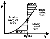
Figure A8. Willingness to Import / Export with Regard to Market Price of Permits.
For whatever market one is considering, we simply add up the quantities (x-axis) potentially supplied and those potentially demanded at each price (y-axis) across the constituent regions. As we vary the price, we describe the demand and the supply curves for this market, and their intersection indicates the market clearing price on the y-axis and the total quantity traded in that market on the x-axis.
Figure A9 shows the aggregate demand and supply curves obtained in the Annex B and world trading cases. The aggregate demand curve is the same in both the Annex B and the global market because both include all Kyoto-constrained, i.e. potentially importing, regions. This single demand curve intersects the horizontal axis at the quantity equal to the sum of the emission reductions required to meet the Kyoto commitments, which is 1.31 Gton. This is the "Kyoto cap" represented by a vertical dotted line on the figure; it is also the quantity of emission permits that would be demanded if the price were $0/ton. At this price, the aggregate supply is the quantity of permits available at no cost. This is the FSU's 111 Mton of hot air.
As the price increases, the demand for permits diminishes, as more and more domestic abatement is undertaken, and the supply of permits increases as more abatement is justified in the unconstrained, exporting regions. As long as the market price is less than the lowest autarkic
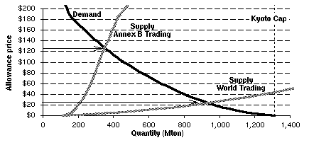
Figure A9. Aggregated Supply and Demand Curves in 2010 under Kytoo Constraints. Annex B Trading / World Trading.
marginal cost for the Kyoto-constrained regions, these regions are always on the demand side; and the unconstrained regions are on the supply side. When the price reaches $116, the marginal cost for EET, this region switches from the demand side to the supply side, resulting in a "kink" on the demand and supply curves (which happens to be almost indiscernible because of the small economic size of this region). Such a kink can readily be seen on both supply and demand curves when the price reaches $186, the autarkic marginal cost for USA. There would be similar kinks at $233 when OOE becomes a supplier and at $273 when the EEC does. At $584, the autarkic marginal cost for Japan meeting the commitment, the demand for permits would be zero.
The following tables show the detailed results for cases studied in the text.
All the prices in the following tables are in 1985$. NAB = Non-Annex B regions
Repeat of Tables Shown in the Text
Basic Cases - Reference Scenario
Basic Cases - Low Growth Scenario
Basic Cases - High Growth Scenario
Import Limitations
CDM Surcharges
Non-Competitive Behavior
Inefficient Supply: Limited to 50% of Full Potential Supply
Other Inefficient Suppy Cases: Limited to 25%, 15%, 10%, 5% of Full Potential Supply
TABLE 1 - bis: Reference emissions and Kyoto commitments
Reference emissions
USA
JPN
EEC
OOE
EET
oecd+eet
FSU
NAB
World
EEX
CHN
IND
DAE
BRA
ROW
Ref 1990 (Mton)
1362
298
822
318
266
3066
891
2022
5979
508
833
183
115
63
320
Ref
2010 (Mton)
1838
424
1064
472
395
4193
763
4142
9098
927
1792
486
308
97
532
low scenario
1748
412
1022
455
375
4012
737
3946
8695
903
1687
457
293
96
510
high scenario
1923
435
1102
488
416
4364
783
4327
9475
950
1891
514
323
98
551
Kyoto
0.93
0.94
0.92
0.95
1.04
\
0.98
\
\
\
\
\
\
\
\
Emissions
in 2010 (Mton)
1267
280
757
301
277
2881
873
4142
7896
927
1792
486
308
97
532
low scenario
1267
280
757
301
277
2881
873
3946
7700
903
1687
457
293
96
510
high scenario
1267
280
757
301
277
2881
873
4327
8081
950
1891
514
323
98
551
Reductions
/ ref 2010 (Mton)
572
144
307
171
118
1312
-111
0
1202
0
0
0
0
0
0
low scenario
481
132
266
154
98
1132
-136
0
995
0
0
0
0
0
0
high scenario
657
155
346
187
139
1484
-90
0
1393
0
0
0
0
0
0
TABLE 2 - bis: MACs approximations coefficients (P = aR2+ bR)
| USA | JPN | EEC | OOE | EET | FSU | EEX | CHN | IND | DAE | BRA | ROW | |
| a | 5.00E-4 | 1.55E-2 | 2.40E-3 | 8.50E-3 | 7.90E-3 | 2.30E-3 | 3.20E-3 | 7.00E-5 | 1.50E-3 | 4.70E-3 | 5.61E-1 | 2.10E-3 |
| b | 0.04 | 1.816 | 0.15 | -0.099 | 0.049 | 0.004 | 0.303 | 0.024 | 0.079 | 0.377 | 8.497 | 0.081 |
BASIC CASES
TABLE A: Kyoto no trading
| USA | JPN | EEC | OOE | EET | oecd+ eet |
FSU | World | |
| Reductions / ref 2010 (Mton) | 572 | 144 | 307 | 171 | 118 | 1312 | 0 | 1312 |
| Marginal Costs ($/ton) | 186 | 584 | 273 | 233 | 116 | \ | \ | \ |
| Cost of Abatement ($billion) | 37.62 | 34.37 | 30.29 | 12.81 | 4.67 | 119.76 | 0.00 | 119.76 |
TABLE B: Annex B trading
| USA | JPN | EEC | OOE | EET | oecd+ eet |
FSU | World | |
| Reductions / ref 2010 (Mton) | 466 | 49 | 201 | 128 | 124 | 968 | 234 | 1202 |
| 'Hot air' (Mton) | \ | \ | \ | \ | \ | 0 | 111 | 111 |
| Permits Market Price ($/ton) | 127 | 127 | 127 | 127 | 127 | 127 | 127 | 127 |
| Cost of Abatement ($billion) | 21.16 | 2.82 | 9.51 | 5.16 | 5.36 | 44.01 | 9.95 | 53.96 |
| Permits exp(-)/imp(+) (Mton) | 106 | 95 | 106 | 43 | -6 | 345 | -345 | 0 |
| i.e % of commitment (import) | 19% | 66% | 35% | 25% | \ | 26% | \ | \ |
| Flows exp(-)/imp(+) ($billion) | 13.44 | 12.06 | 13.51 | 5.49 | -0.73 | 43.77 | -43.77 | 0.00 |
| Total Cost ($billion) | 34.60 | 14.88 | 23.02 | 10.64 | 4.64 | 87.78 | -33.82 | 53.96 |
| Gains from trade ($billion) | 3.03 | 19.49 | 7.27 | 2.17 | 0.03 | 31.99 | 33.82 | 65.81 |
TABLE C: World trading
| USA | JPN | EEC | OOE | EET | oecd+eet | FSU | NAB | World | EEX | CHN | IND | DAE | BRA | ROW | |
| Reductions / ref 2010 (Mton) | 182 | 12 | 73 | 59 | 52 | 378 | 101 | 723 | 1202 | 51 | 437 | 102 | 42 | 2 | 89 |
| 'Hot air' (Mton) | \ | \ | \ | \ | \ | 0 | 111 | 0 | 111 | \ | \ | \ | \ | \ | \ |
| Permits Market Price ($/ton) | 24 | 24 | 24 | 24 | 24 | 24 | 24 | 24 | 24 | 24 | 24 | 24 | 24 | 24 | 24 |
| Cost of Abatement ($billion) | 1.66 | 0.14 | 0.71 | 0.41 | 0.43 | 3.36 | 0.81 | 6.99 | 11.15 | 0.54 | 4.22 | 0.95 | 0.44 | 0.03 | 0.81 |
| Permits exp(-)/imp(+) (Mton) | 390 | 132 | 234 | 112 | 66 | 935 | -211 | -723 | 0 | -51 | -437 | -102 | -42 | -2 | -89 |
| i.e % of commitment (import) | 68% | 92% | 76% | 66% | 56% | 71% | \ | \ | \ | \ | \ | \ | \ | \ | \ |
| Flows exp(-)/imp(+) ($billion) | 9.27 | 3.15 | 5.57 | 2.67 | 1.57 | 22.24 | -5.03 | -17.21 | 0.00 | -1.21 | -10.40 | -2.44 | -0.99 | -0.06 | -2.12 |
| Total Cost ($billion) | 10.94 | 3.29 | 6.29 | 3.09 | 2.01 | 25.60 | -4.22 | -10.22 | 11.15 | -0.68 | -6.17 | -1.49 | -0.55 | -0.03 | -1.31 |
| Gains from trade ($billion) | 26.69 | 31.08 | 24.00 | 9.73 | 2.66 | 94.16 | 4.22 | 10.22 | 108.61 | 0.68 | 6.17 | 1.49 | 0.55 | 0.03 | 1.31 |
BASIC CASES, low scenario
TABLE A': Kyoto no trading
| USA | JPN | EEC | OOE | EET | oecd+ eet |
FSU | World | |
| Reductions / ref 2010 (Mton) | 481 | 132 | 266 | 154 | 98 | 1132 | 0 | 1132 |
| Marginal Costs ($/ton) | 135 | 510 | 210 | 187 | 81 | \ | \ | \ |
| Cost of Abatement ($billion) | 23.19 | 27.74 | 20.36 | 9.24 | 2.71 | 83.24 | 0.00 | 83.24 |
TABLE B': Annex B trading
| USA | JPN | EEC | OOE | EET | oecd+ eet |
FSU | World | |
| Reductions / ref 2010 (Mton) | 385 | 37 | 164 | 109 | 103 | 799 | 196 | 995 |
| 'Hot air' (Mton) | \ | \ | \ | \ | \ | 0 | 136 | 136 |
| Permits Market Price ($/ton) | 90 | 90 | 90 | 90 | 90 | 90 | 90 | 90 |
| Cost of Abatement ($billion) | 12.47 | 1.54 | 5.58 | 3.05 | 3.17 | 25.81 | 5.88 | 31.69 |
| Permits exp(-)/imp(+) (Mton) | 96 | 95 | 102 | 46 | -5 | 333 | -333 | 0 |
| i.e % of commitment (import) | 20% | 72% | 38% | 30% | \ | 29% | \ | \ |
| Flows exp(-)/imp(+) ($billion) | 8.60 | 8.48 | 9.10 | 4.10 | -0.48 | 29.79 | -29.79 | 0.00 |
| Total Cost ($billion) | 21.08 | 10.01 | 14.67 | 7.14 | 2.69 | 55.59 | -23.90 | 31.69 |
| Gains from trade ($billion) | 2.11 | 17.73 | 5.69 | 2.10 | 0.02 | 27.65 | 23.90 | 51.55 |
TABLE C': World trading
| USA | JPN | EEC | OOE | EET | oecd+eet | FSU | NAB | World | EEX | CHN | IND | DAE | BRA | ROW | |
| Reductions / ref 2010 (Mton) | 152 | 9 | 60 | 52 | 44 | 316 | 86 | 593 | 995 | 41 | 358 | 85 | 33 | 2 | 74 |
| 'Hot air' (Mton) | \ | \ | \ | \ | \ | 0 | 136 | 0 | 136 | \ | \ | \ | \ | \ | \ |
| Permits Market Price ($/ton) | 18 | 18 | 18 | 18 | 18 | 18 | 18 | 18 | 18 | 18 | 18 | 18 | 18 | 18 | 18 |
| Cost of Abatement ($billion) | 1.04 | 0.08 | 0.44 | 0.26 | 0.27 | 2.09 | 0.51 | 4.30 | 6.90 | 0.32 | 2.60 | 0.59 | 0.26 | 0.02 | 0.51 |
| Permits exp(-)/imp(+) (Mton) | 330 | 123 | 206 | 103 | 54 | 816 | -223 | -593 | 0 | -41 | -358 | -85 | -33 | -2 | -74 |
| i.e % of commitment (import) | 68% | 93% | 78% | 67% | 55% | 72% | \ | \ | \ | \ | \ | \ | \ | \ | \ |
| Flows exp(-)/imp(+) ($billion) | 5.78 | 2.16 | 3.62 | 1.80 | 0.94 | 14.30 | -3.91 | -10.40 | 0.00 | -0.71 | -6.28 | -1.49 | -0.58 | -0.03 | -1.30 |
| Total Cost ($billion) | 6.82 | 2.24 | 4.06 | 2.06 | 1.22 | 16.39 | -3.40 | -6.10 | 6.90 | -0.39 | -3.68 | -0.90 | -0.32 | -0.02 | -0.79 |
| Gains from trade ($billion) | 16.37 | 25.50 | 16.31 | 7.18 | 1.49 | 66.85 | 3.40 | 6.10 | 76.35 | 0.39 | 3.68 | 0.90 | 0.32 | 0.02 | 0.79 |
BASIC CASES, high scenario
TABLE A'': Kyoto no trading
| USA | JPN | EEC | OOE | EET | oecd+ eet |
FSU | World | |
| Reductions / ref 2010 (Mton) | 657 | 155 | 346 | 187 | 139 | 1484 | 0 | 1484 |
| Marginal Costs ($/ton) | 242 | 656 | 339 | 279 | 159 | \ | \ | \ |
| Cost of Abatement ($billion) | 55.77 | 41.28 | 42.00 | 16.83 | 7.53 | 163.41 | 0.00 | 163.41 |
TABLE B'': Annex B trading
| USA | JPN | EEC | OOE | EET | oecd+ eet |
FSU | World | |
| Reductions / ref 2010 (Mton) | 540 | 61 | 235 | 146 | 143 | 1124 | 269 | 1393 |
| 'Hot air' (Mton) | \ | \ | \ | \ | \ | 0 | 90 | 90 |
| Permits Market Price ($/ton) | 167 | 167 | 167 | 167 | 167 | 167 | 167 | 167 |
| Cost of Abatement ($billion) | 32.09 | 4.51 | 14.48 | 7.81 | 8.12 | 67.00 | 15.06 | 82.06 |
| Permits exp(-)/imp(+) (Mton) | 116 | 95 | 111 | 41 | -4 | 359 | -359 | 0 |
| i.e % of commitment (import) | 18% | 61% | 32% | 22% | \ | 24% | \ | \ |
| Flows exp(-)/imp(+) ($billion) | 19.49 | 15.84 | 18.57 | 6.84 | -0.61 | 60.14 | -60.14 | 0.00 |
| Total Cost ($billion) | 51.58 | 20.35 | 33.05 | 14.65 | 7.51 | 127.14 | -45.08 | 82.06 |
| Gains from trade ($billion) | 4.19 | 20.93 | 8.95 | 2.18 | 0.01 | 36.27 | 45.08 | 81.36 |
TABLE C'': World trading
| USA | JPN | EEC | OOE | EET | oecd+ eet |
FSU | NAB | World | EEX | CHN | IND | DAE | BRA | ROW | |
| Reductions / ref 2010 (Mton) | 210 | 15 | 85 | 66 | 59 | 435 | 114 | 844 | 1393 | 61 | 510 | 118 | 50 | 3 | 103 |
| 'Hot air' (Mton) | \ | \ | \ | \ | \ | 0 | 90 | 0 | 90 | \ | \ | \ | \ | \ | \ |
| Permits Market Price ($/ton) | 30 | 30 | 30 | 30 | 30 | 30 | 30 | 30 | 30 | 30 | 30 | 30 | 30 | 30 | 30 |
| Cost of Abatement ($billion) | 2.42 | 0.22 | 1.05 | 0.60 | 0.63 | 4.90 | 1.16 | 10.26 | 16.33 | 0.80 | 6.19 | 1.38 | 0.66 | 0.04 | 1.18 |
| Permits exp(-)/imp(+) (Mton) | 447 | 141 | 260 | 121 | 80 | 1049 | -204 | -844 | 0 | -61 | -510 | -118 | -50 | -3 | -103 |
| i.e % of commitment (import) | 68% | 90% | 75% | 65% | 58% | 71% | \ | \ | \ | \ | \ | \ | \ | \ | \ |
| Flows exp(-)/imp(+) ($billion) | 13.57 | 4.27 | 7.90 | 3.68 | 2.43 | 31.84 | -6.20 | -25.64 | 0.00 | -1.85 | -15.47 | -3.60 | -1.51 | -0.09 | -3.11 |
| Total Cost ($billion) | 15.98 | 4.48 | 8.95 | 4.28 | 3.05 | 36.74 | -5.04 | -15.37 | 16.33 | -1.05 | -9.28 | -2.21 | -0.85 | -0.05 | -1.94 |
| Gains from trade ($billion) | 39.79 | 36.80 | 33.05 | 12.56 | 4.48 | 126.67 | 5.04 | 15.37 | 147.09 | 1.05 | 9.28 | 2.21 | 0.85 | 0.05 | 1.94 |
IMPORT LIMITATIONS
TABLE D: 75%
| USA | JPN | EEC | OOE | EET | oecd+eet | FSU | NAB | World | EEX | CHN | IND | DAE | BRA | ROW | |
| Reductions / ref 2010 (Mton) | 178 | 36 | 77 | 58 | 51 | 399 | 99 | 704 | 1202 | 49 | 425 | 100 | 40 | 2 | 87 |
| 'Hot air' (Mton) | \ | \ | \ | \ | \ | 0 | 111 | 0 | 111 | \ | \ | \ | \ | \ | \ |
| Permits Market Price ($/ton) | 23 | 23 | 23 | 23 | 23 | 23 | 23 | 23 | 23 | 23 | 23 | 23 | 23 | 23 | 23 |
| Cost of Abatement ($billion) | 1.56 | 1.42 | 0.81 | 0.39 | 0.41 | 4.58 | 0.76 | 6.54 | 11.88 | 0.50 | 3.96 | 0.89 | 0.41 | 0.03 | 0.76 |
| Permits exp(-)/imp(+) (Mton) | 394 | 108 | 230 | 113 | 67 | 913 | -209 | -704 | 0 | -49 | -425 | -100 | -40 | -2 | -87 |
| i.e % of commitment (import) | 69% | 75% | 75% | 66% | 57% | 68% | \ | \ | \ | \ | \ | \ | \ | \ | \ |
| Flows exp(-)/imp(+) ($billion) | 8.99 | 2.47 | 5.26 | 2.59 | 1.54 | 20.84 | -4.77 | -16.07 | 0.00 | -1.13 | -9.70 | -2.28 | -0.92 | -0.05 | -1.98 |
| Total Cost ($billion) | 10.55 | 3.89 | 6.06 | 2.97 | 1.94 | 25.42 | -4.02 | -9.52 | 11.88 | -0.63 | -5.75 | -1.39 | -0.51 | -0.03 | -1.22 |
| Gains from trade ($billion) | 27.07 | 30.48 | 24.22 | 9.84 | 2.73 | 94.34 | 4.02 | 9.52 | 107.88 | 0.63 | 5.75 | 1.39 | 0.51 | 0.03 | 1.22 |
| D gain in % / no limit (table C) | 1 | -2 | 1 | 1 | 2 | 0 | -5 | -7 | -1 | -7 | -7 | -7 | -7 | -8 | -7 |
TABLE E: 50%
| USA | JPN | EEC | OOE | EET | oecd+eet | FSU | NAB | World | EEX | CHN | IND | DAE | BRA | ROW | |
| Reductions / ref 2010 (Mton) | 286 | 72 | 154 | 86 | 59 | 656 | 73 | 473 | 1202 | 31 | 286 | 69 | 25 | 1 | 60 |
| 'Hot air' (Mton) | \ | \ | \ | \ | \ | 0 | 111 | 0 | 111 | \ | \ | \ | \ | \ | \ |
| Permits Market Price ($/ton) | 13 | 13 | 13 | 13 | 13 | 13 | 13 | 13 | 13 | 13 | 13 | 13 | 13 | 13 | $13 |
| Cost of Abatement ($billion) | 5.52 | 6.66 | 4.67 | 1.42 | 0.63 | 18.89 | 0.31 | 2.50 | 21.70 | 0.18 | 1.52 | 0.35 | 0.15 | 0.01 | 0.30 |
| Permits exp(-)/imp(+) (Mton) | 286 | 72 | 154 | 86 | 59 | 656 | -183 | -473 | 0 | -31 | -286 | -69 | -25 | -1 | -60 |
| i.e % of commitment (import) | 50% | 50% | 50% | 50% | 50% | 49% | \ | \ | \ | \ | \ | \ | \ | \ | \ |
| Flows exp(-)/imp(+) ($billion) | 3.58 | 0.90 | 1.93 | 1.07 | 0.74 | 8.23 | -2.30 | -5.93 | 0.00 | -0.39 | -3.58 | -0.86 | -0.32 | -0.02 | -0.76 |
| Total Cost ($billion) | 9.10 | 7.56 | 6.60 | 2.50 | 1.37 | 27.12 | -1.99 | -3.42 | 21.70 | -0.21 | -2.06 | -0.51 | -0.17 | -0.01 | -0.46 |
| Gains from trade ($billion) | 28.53 | 26.81 | 23.69 | 10.32 | 3.30 | 92.64 | 1.99 | 3.42 | 98.06 | 0.21 | 2.06 | 0.51 | 0.17 | 0.01 | 0.46 |
| D gain in % / no limit (table C) | 7 | -14 | -1 | 6 | 24 | -2 | -53 | -67 | -10 | -69 | -67 | -65 | -69 | -71 | -65 |
TABLE F: 25%
| USA | JPN | EEC | OOE | EET | oecd+eet | FSU | NAB | World | EEX | CHN | IND | DAE | BRA | ROW | |
| Reductions / ref 2010 (Mton) | 429 | 108 | 230 | 129 | 89 | 984 | 38 | 180 | 1202 | 10 | 108 | 28 | 8 | 0 | 25 |
| 'Hot air' (Mton) | \ | \ | \ | \ | \ | 0 | 111 | 0 | 111 | \ | \ | \ | \ | \ | \ |
| Permits Market Price ($/ton) | 3 | 3 | 3 | 3 | 3 | 3 | 3 | 3 | 3 | 3 | 3 | 3 | 3 | 3 | 3 |
| Cost of Abatement ($billion) | 16.79 | 17.15 | 13.77 | 5.20 | 2.02 | 54.94 | 0.04 | 0.28 | 55.26 | 0.02 | 0.17 | 0.04 | 0.01 | 0.00 | 0.04 |
| Permits exp(-)/imp(+) (Mton) | 143 | 36 | 77 | 43 | 30 | 328 | -148 | -180 | 0 | -10 | -108 | -28 | -8 | 0 | -25 |
| i.e % of commitment (import) | 25% | 25% | 25% | 25% | 25% | 24% | \ | \ | \ | \ | \ | \ | \ | \ | \ |
| Flows exp(-)/imp(+) ($billion) | 0.48 | 0.12 | 0.26 | 0.15 | 0.10 | 1.11 | -0.50 | -0.61 | 0.00 | -0.03 | -0.37 | -0.10 | -0.03 | 0.00 | -0.09 |
| Total Cost ($billion) | 17.27 | 17.28 | 14.04 | 5.35 | 2.12 | 56.05 | -0.46 | -0.33 | 55.26 | -0.02 | -0.20 | -0.05 | -0.01 | 0.00 | -0.05 |
| Gains from trade ($billion) | 20.35 | 17.09 | 16.25 | 7.47 | 2.55 | 63.72 | 0.46 | 0.33 | 64.51 | 0.02 | 0.20 | 0.05 | 0.01 | 0.00 | 0.05 |
| D gain in % / no limit (table C) | -24 | -45 | -32 | -23 | -4 | -32 | -89 | -97 | -41 | -97 | -97 | -96 | -97 | -98 | -96 |
CDM SURCHARGES
TABLE G: 25%
| USA | JPN | EEC | OOE | EET | oecd+eet | FSU | NAB | World | EEX | CHN | IND | DAE | BRA | ROW | |
| Reductions / ref 2010 (Mton) | 198 | 14 | 80 | 63 | 56 | 410 | 108 | 687 | 1205 | 48 | 415 | 98 | 39 | 2 | 85 |
| 'Hot air' (Mton) | \ | \ | \ | \ | \ | 0 | 111 | 0 | 111 | \ | \ | \ | \ | \ | \ |
| Permits Market Price ($/ton) | 27 | 27 | 27 | 27 | 27 | 27 | 27 | 22 | \ | 22 | 22 | 22 | 22 | 22 | 22 |
| Cost of Abatement ($billion) | 2.07 | 0.18 | 0.89 | 0.51 | 0.54 | 4.19 | 1.00 | 6.15 | 11.34 | 0.47 | 3.72 | 0.84 | 0.38 | 0.02 | 0.72 |
| Permits exp(-)/imp(+) (Mton) | 374 | 131 | 227 | 108 | 62 | 902 | -219 | -687 | -3 | -48 | -415 | -98 | -39 | -2 | -85 |
| i.e % of commitment (import) | 65% | 91% | 74% | 63% | 53% | 67% | \ | \ | \ | \ | \ | \ | \ | \ | \ |
| Flows exp(-)/imp(+) ($billion) | 10.26 | 3.58 | 6.23 | 2.98 | 1.70 | 24.75 | -6.01 | -15.07 | 3.68 | -1.05 | -9.10 | -2.14 | -0.86 | -0.05 | -1.86 |
| Total Cost ($billion) | 12.32 | 3.76 | 7.13 | 3.49 | 2.24 | 28.94 | -5.01 | -8.92 | 15.02 | -0.59 | -5.38 | -1.30 | -0.48 | -0.03 | -1.15 |
| Gains from trade ($billion) | 25.30 | 30.60 | 23.16 | 9.33 | 2.43 | 90.82 | 5.01 | 8.92 | 104.75 | 0.59 | 5.38 | 1.30 | 0.48 | 0.03 | 1.15 |
| D gain in % / no limit (table C) | -5 | -2 | -3 | -4 | -9 | -4 | 19 | -13 | -4 | -14 | -13 | -12 | -14 | -14 | -12 |
TABLE H: 50%
| USA | JPN | EEC | OOE | EET | oecd+eet | FSU | NAB | World | EEX | CHN | IND | DAE | BRA | ROW | |
| Reductions / ref 2010 (Mton) | 211 | 15 | 86 | 66 | 59 | 436 | 114 | 654 | 1205 | 45 | 395 | 93 | 37 | 2 | 81 |
| 'Hot air' (Mton) | \ | \ | \ | \ | \ | 0 | 111 | 0 | 111 | \ | \ | \ | \ | \ | \ |
| Permits Market Price ($/ton) | 31 | 31 | 31 | 31 | 31 | 31 | 31 | 20 | \ | 20 | 20 | 20 | 20 | 20 | 20 |
| Cost of Abatement ($billion) | 2.44 | 0.22 | 1.06 | 0.60 | 0.63 | 4.95 | 1.17 | 5.46 | 11.58 | 0.41 | 3.30 | 0.75 | 0.34 | 0.02 | 0.64 |
| Permits exp(-)/imp(+) (Mton) | 361 | 129 | 221 | 105 | 59 | 876 | -225 | -654 | -3 | -45 | -395 | -93 | -37 | -2 | -81 |
| i.e % of commitment (import) | 63% | 90% | 72% | 61% | 50% | 65% | \ | \ | \ | \ | \ | \ | \ | \ | \ |
| Flows exp(-)/imp(+) ($billion) | 11.03 | 3.95 | 6.76 | 3.22 | 1.80 | 26.76 | -6.87 | -13.32 | 6.57 | -0.93 | -8.05 | -1.90 | -0.75 | -0.04 | -1.65 |
| Total Cost ($billion) | 13.47 | 4.17 | 7.82 | 3.82 | 2.43 | 31.71 | -5.70 | -7.86 | 18.15 | -0.51 | -4.74 | -1.15 | -0.42 | -0.02 | -1.01 |
| Gains from trade ($billion) | 24.16 | 30.20 | 22.46 | 9.00 | 2.24 | 88.06 | 5.70 | 7.86 | 101.61 | 0.51 | 4.74 | 1.15 | 0.42 | 0.02 | 1.01 |
| D gain in % / no limit (table C) | -9 | -3 | -6 | -8 | -16 | -6 | 35 | -23 | -6 | -24 | -23 | -23 | -24 | -26 | -22% |
TABLE I: 100%
| USA | JPN | EEC | OOE | EET | oecd+eet | FSU | NAB | World | EEX | CHN | IND | DAE | BRA | ROW | |
| Reductions / ref 2010 (Mton) | 231 | 17 | 95 | 71 | 64 | 479 | 124 | 602 | 1204 | 41 | 364 | 86 | 34 | 2 | 75 |
| 'Hot air' (Mton) | \ | \ | \ | \ | \ | 0 | 111 | 0 | 111 | \ | \ | \ | \ | \ | \ |
| Permits Market Price ($/ton) | 36 | 36 | 36 | 36 | 36 | 36 | 36 | 18 | \ | 18 | 18 | 18 | 18 | 18 | 18 |
| Cost of Abatement ($billion) | 3.12 | 0.30 | 1.36 | 0.77 | 0.80 | 6.34 | 1.49 | 4.46 | 12.30 | 0.33 | 2.70 | 0.61 | 0.27 | 0.02 | 0.53 |
| Permits exp(-)/imp(+) (Mton) | 341 | 127 | 212 | 100 | 54 | 834 | -235 | -602 | -2 | -41 | -364 | -86 | -34 | -2 | -75 |
| i.e % of commitment (import) | 60% | 88% | 69% | 59% | 45% | 62% | \ | \ | \ | \ | \ | \ | \ | \ | \ |
| Flows exp(-)/imp(+) ($billion) | 12.22 | 4.56 | 7.62 | 3.60 | 1.93 | 29.92 | -8.41 | -10.79 | 10.71 | -0.74 | -6.52 | -1.55 | -0.60 | -0.03 | -1.35 |
| Total Cost ($billion) | 15.34 | 4.85 | 8.98 | 4.37 | 2.73 | 36.26 | -6.92 | -6.33 | 23.01 | -0.41 | -3.82 | -0.93 | -0.33 | -0.02 | -0.82 |
| Gains from trade ($billion) | 22.29 | 29.52 | 21.31 | 8.45 | 1.94 | 83.50 | 6.92 | 6.33 | 96.76 | 0.41 | 3.82 | 0.93 | 0.33 | 0.02 | 0.82 |
| Dgain in % / no limit (table C) | -16 | -5 | -11 | -13 | -27 | -11 | 64 | -38 | -11 | -40 | -38 | -37 | -40 | -42 | -37 |
NON-COMPETITIVE BEHAVIOR
TABLE J: World trading, CDM monopoly
| USA | JPN | EEC | OOE | EET | oecd+eet | FSU | NAB | World | EEX | CHN | IND | DAE | BRA | ROW | |
| Reductions / ref 2010 (Mton) | 317 | 28 | 133 | 92 | 86 | 656 | 164 | 382 | 1202 | 24 | 230 | 56 | 20 | 1 | 50 |
| 'Hot air' (Mton) | \ | \ | \ | \ | \ | 0 | 111 | 0 | 111 | \ | \ | \ | \ | \ | \ |
| PermitsMarket Price ($/ton) | 63 | 63 | 63 | 63 | 63 | 63 | 63 | 63 | 63 | 63 | 63 | 63 | 63 | 63 | 63 |
| Cost of Abatement ($billion) | 7.29 | 0.82 | 3.24 | 1.78 | 1.86 | 14.99 | 3.45 | 1.52 | 19.96 | 0.10 | 0.92 | 0.22 | 0.08 | 0.00 | 0.19 |
| Permits exp(-)/imp(+) (Mton) | 255 | 116 | 174 | 79 | 32 | 656 | -275 | -382 | 0 | -24 | -230 | -56 | -20 | -1 | -50 |
| i.e % of commitment (import) | 45% | 81% | 57% | 46% | 27% | 50% | \ | \ | \ | \ | \ | \ | \ | \ | \ |
| Flows exp(-)/imp(+) ($billion) | 15.99 | 7.30 | 10.91 | 4.99 | 2.00 | 41.19 | -17.24 | -23.94 | 0.00 | -1.52 | -14.46 | -3.54 | -1.23 | -0.06 | -3.13 |
| Total Cost ($billion) | 23.28 | 8.12 | 14.14 | 6.77 | 3.86 | 56.17 | -13.79 | -22.43 | 19.96 | -1.42 | -13.54 | -3.33 | -1.15 | -0.06 | -2.94 |
| Gains from trade ($billion) | 14.34 | 26.25 | 16.15 | 6.05 | 0.80 | 63.59 | 13.79 | 22.43 | 99.81 | 1.42 | 13.54 | 3.33 | 1.15 | 0.06 | 2.94 |
TABLE K: World trading, CDM+FSU monopoly
| USA | JPN | EEC | OOE | EET | oecd+eet | FSU | NAB | World | EEX | CHN | IND | DAE | BRA | ROW | |
| Reductions / ref 2010 (Mton) | 417 | 42 | 179 | 116 | 112 | 866 | 51 | 285 | 1202 | 17 | 172 | 43 | 14 | 1 | 38 |
| 'Hot air' (Mton) | \ | \ | \ | \ | \ | 0 | 111 | 0 | 111 | \ | \ | \ | \ | \ | \ |
| Permits Market Price ($/ton) | 108 | 108 | 108 | 108 | 108 | 108 | 108 | 108 | 108 | 108 | 108 | 108 | 108 | 108 | 108 |
| Cost of Abatement ($billion) | 15.58 | 1.99 | 6.99 | 3.80 | 3.96 | 32.31 | 0.11 | 0.77 | 33.20 | 0.05 | 0.47 | 0.11 | 0.04 | 0.00 | 0.10 |
| Permits exp(-)/imp(+) (Mton) | 154 | 102 | 128 | 55 | 7 | 446 | -161 | -285 | 0 | -17 | -172 | -43 | -14 | -1 | -38 |
| i.e % of commitment (import) | 27% | 71% | 42% | 32% | 6% | 34% | \ | \ | \ | \ | \ | \ | \ | \ | \ |
| Flows exp(-)/imp(+) ($billion) | 16.69 | 11.06 | 13.89 | 5.95 | 0.70 | 48.29 | -17.47 | -30.82 | 0.00 | -1.86 | -18.58 | -4.66 | -1.51 | -0.08 | -4.15 |
| Total Cost ($billion) | 32.28 | 13.05 | 20.87 | 9.75 | 4.66 | 80.61 | -17.36 | -30.05 | 33.20 | -1.81 | -18.11 | -4.54 | -1.47 | -0.07 | -4.05 |
| Gains from trade ($billion) | 5.35 | 21.32 | 9.41 | 3.06 | 0.01 | 39.16 | 17.36 | 30.05 | 86.57 | 1.81 | 18.11 | 4.54 | 1.47 | 0.07 | 4.05 |
TABLE L: 50% - CDM+FSU monopoly
| USA | JPN | EEC | OOE | EET | oecd+eet | FSU | NAB | World | EEX | CHN | IND | DAE | BRA | ROW | |
| Reductions / ref 2010 (Mton) | 417 | 72 | 179 | 116 | 111 | 895 | 48 | 259 | 1202 | 15 | 156 | 39 | 12 | 1 | 35 |
| 'Hot air' (Mton) | \ | \ | \ | \ | \ | 0 | 111 | 0 | 111 | \ | \ | \ | \ | \ | \ |
| Permits Market Price ($/ton) | 103 | 103 | 103 | 103 | 103 | 103 | 103 | 103 | 103 | 103 | 103 | 103 | 103 | 103 | 103 |
| Cost of Abatement ($billion) | 15.52 | 6.66 | 6.96 | 3.78 | 3.94 | 36.85 | 0.09 | 0.63 | 37.56 | 0.04 | 0.38 | 0.09 | 0.03 | 0.00 | 0.08 |
| Permits exp(-)/imp(+) (Mton) | 155 | 72 | 129 | 55 | 7 | 417 | -158 | -259 | 0 | -15 | -156 | -39 | -12 | -1 | -35 |
| i.e % of commitment (import) | 27% | 50% | 42% | 32% | 6% | 31% | \ | \ | \ | \ | \ | \ | \ | \ | \ |
| Flows exp(-)/imp(+) ($billion) | 16.02 | 7.46 | 13.30 | 5.70 | 0.69 | 43.16 | -16.36 | -26.80 | 0.00 | -1.60 | -16.14 | -4.08 | -1.29 | -0.06 | -3.64 |
| Total Cost ($billion) | 31.53 | 14.11 | 20.25 | 9.49 | 4.63 | 80.01 | -16.27 | -26.17 | 37.56 | -1.56 | -15.76 | -3.98 | -1.26 | -0.06 | -3.56 |
| Gains from trade ($billion) | 6.09 | 20.26 | 10.03 | 3.33 | 0.04 | 39.75 | 16.27 | 26.17 | 82.20 | 1.56 | 15.76 | 3.98 | 1.26 | 0.06 | 3.56 |
| D gain in % / no limit (table C) | -77 | -35 | -58 | -66 | -98 | -58 | 285 | 156 | -24 | 129 | 155 | 168 | 128 | 106 | 173 |
INEFFICIENT SUPPLY - 50%
TABLE M: competitive case
| USA | JPN | EEC | OOE | EET | oecd+eet | FSU | NAB | World | EEX | CHN | IND | DAE | BRA | ROW | |
| Reductions / ref 2010 (Mton) | 286 | 24 | 120 | 84 | 78 | 593 | 75 | 590 | 1257 | 45 | 355 | 81 | 36 | 2 | 70 |
| 'Hot air' (Mton) | \ | \ | \ | \ | \ | 0 | 55 | 0 | 55 | \ | \ | \ | \ | \ | \ |
| Permits Market Price ($/ton) | 52 | 52 | 52 | 52 | 52 | 52 | 52 | 52 | 52 | 52 | 52 | 52 | 52 | 52 | 52 |
| Cost of Abatement ($billion) | 5.53 | 0.59 | 2.45 | 1.36 | 1.42 | 11.34 | 1.32 | 11.98 | 24.63 | 0.98 | 7.20 | 1.59 | 0.80 | 0.06 | 1.35 |
| Permits exp(-)/imp(+) (Mton) | 285 | 120 | 188 | 87 | 40 | 720 | -130 | -590 | 0 | -45 | -355 | -81 | -36 | -2 | -70 |
| i.e % of commitment (import) | 50% | 83% | 61% | 51% | 34% | 55% | \ | \ | \ | \ | \ | \ | \ | \ | \ |
| Flows exp(-)/imp(+) ($billion) | 14.94 | 6.29 | 9.82 | 4.55 | 2.08 | 37.67 | -6.82 | -30.86 | 0.00 | -2.33 | -18.59 | -4.25 | -1.90 | -0.12 | -3.66 |
| Total Cost ($billion) | 20.47 | 6.88 | 12.26 | 5.90 | 3.49 | 49.01 | -5.50 | -18.88 | 24.63 | -1.35 | -11.39 | -2.66 | -1.10 | -0.07 | -2.31 |
| Gains from trade ($billion) | 17.15 | 27.48 | 18.03 | 6.91 | 1.18 | 70.75 | 5.50 | 18.88 | 95.13 | 1.35 | 11.39 | 2.66 | 1.10 | 0.07 | 2.31 |
| D gain in % / no limit (table C) | -36 | -12 | -25 | -29 | -56 | -25 | 30 | 85 | -12 | 99 | 85 | 79 | 100 | 121 | 77 |
TABLE N: CDM monopoly
| USA | JPN | EEC | OOE | EET | oecd+eet | FSU | NAB | World | EEX | CHN | IND | DAE | BRA | ROW | |
| Reductions / ref 2010 (Mton) | 385 | 37 | 164 | 109 | 103 | 799 | 98 | 360 | 1257 | 25 | 217 | 51 | 21 | 1 | 44 |
| 'Hot air' (Mton) | \ | \ | \ | \ | \ | 0 | 55 | 0 | 55 | \ | \ | \ | \ | \ | \ |
| Permits Market Price ($/ton) | 90 | 90 | 90 | 90 | 90 | 90 | 90 | 90 | 90 | 90 | 90 | 90 | 90 | 90 | 90 |
| Cost of Abatement ($billion) | 12.48 | 1.54 | 5.58 | 3.05 | 3.17 | 25.83 | 2.94 | 3.45 | 32.22 | 0.26 | 2.09 | 0.47 | 0.22 | 0.01 | 0.40 |
| Permits exp(-)/imp(+) (Mton) | 186 | 107 | 143 | 63 | 15 | 513 | -153 | -360 | 0 | -25 | -217 | -51 | -21 | -1 | -44 |
| i.e % of commitment (import) | 33% | 74% | 46% | 37% | 12% | 39% | \ | \ | \ | \ | \ | \ | \ | \ | \ |
| Flows exp(-)/imp(+) ($billion) | 16.68 | 9.56 | 12.79 | 5.62 | 1.31 | 45.97 | -13.74 | -32.23 | 0.00 | -2.27 | -19.46 | -4.57 | -1.85 | -0.11 | -3.97 |
| Total Cost ($billion) | 29.17 | 11.10 | 18.37 | 8.67 | 4.48 | 71.79 | -10.80 | -28.77 | 32.22 | -2.01 | -17.38 | -4.10 | -1.63 | -0.09 | -3.57 |
| Gains from trade ($billion) | 8.46 | 23.27 | 11.91 | 4.15 | 0.19 | 47.97 | 10.80 | 28.77 | 87.54 | 2.01 | 17.38 | 4.10 | 1.63 | 0.09 | 3.57 |
| Dgain in % / no limit (table C) | -68 | -25 | -50 | -57 | -93 | -49 | 156 | 181 | -19 | 196 | 182 | 175 | 197 | 212 | 173 |
TABLE O: CDM+FSU monopoly
| USA | JPN | EEC | OOE | EET | oecd+eet | FSU | NAB | World | EEX | CHN | IND | DAE | BRA | ROW | |
| Reductions / ref 2010 (Mton) | 434 | 45 | 187 | 121 | 116 | 902 | 45 | 310 | 1257 | 21 | 187 | 44 | 17 | 1 | 39 |
| 'Hot air' (Mton) | \ | \ | \ | \ | \ | 0 | 55 | 0 | 55 | \ | \ | \ | \ | \ | \ |
| Permits Market Price ($/ton) | 112 | 112 | 112 | 112 | 112 | 112 | 112 | 112 | 112 | 112 | 112 | 112 | 112 | 112 | 112 |
| Cost of Abatement ($billion) | 17.43 | 2.26 | 7.82 | 4.25 | 4.42 | 36.18 | 0.28 | 2.40 | 38.87 | 0.18 | 1.45 | 0.33 | 0.15 | 0.01 | 0.28 |
| Permits exp(-)/imp(+) (Mton) | 137 | 100 | 121 | 51 | 2 | 410 | -100 | -310 | 0 | -21 | -187 | -44 | -17 | -1 | -39 |
| i.e % of commitment (import) | 24% | 69% | 39% | 30% | 2% | 31% | \ | \ | \ | \ | \ | \ | \ | \ | \ |
| Flows exp(-)/imp(+) ($billion) | 15.31 | 11.13 | 13.46 | 5.67 | 0.24 | 45.82 | -11.17 | -34.65 | 0.00 | -2.39 | -20.94 | -4.96 | -1.94 | -0.11 | -4.32 |
| Total Cost ($billion) | 32.74 | 13.39 | 21.29 | 9.92 | 4.67 | 82.00 | -10.89 | -32.25 | 38.87 | -2.21 | -19.48 | -4.63 | -1.79 | -0.10 | -4.04 |
| Gains from trade ($billion) | 4.89 | 20.98 | 9.00 | 2.89 | 0.00 | 37.76 | 10.89 | 32.25 | 80.90 | 2.21 | 19.48 | 4.63 | 1.79 | 0.10 | 4.04 |
| D gain in % / no limit (table C) | -82 | -33 | -62 | -70 | -100 | -60 | 158 | 215 | -26 | 225 | 216 | 211 | 226 | 234 | 209 |
TABLE P: competitive case - with 50% limitation on imports
| USA | JPN | EEC | OOE | EET | oecd+eet | FSU | NAB | World | EEX | CHN | IND | DAE | BRA | ROW | |
| Reductions / ref 2010 (Mton) | 286 | 72 | 154 | 86 | 71 | 668 | 68 | 522 | 1257 | 39 | 315 | 72 | 32 | 2 | 62 |
| 'Hot air' (Mton) | \ | \ | \ | \ | \ | 0 | 55 | 0 | 55 | \ | \ | \ | \ | \ | \ |
| Permits Market Price ($/ton) | 43 | 43 | 43 | 43 | 43 | 43 | 43 | 43 | 43 | 43 | 43 | 43 | 43 | 43 | 43 |
| Cost of Abatement ($billion) | 5.52 | 6.66 | 4.67 | 1.42 | 1.05 | 19.31 | 0.97 | 8.75 | 29.03 | 0.70 | 5.27 | 1.17 | 0.58 | 0.04 | 0.99 |
| Permits exp(-)/imp(+) (Mton) | 286 | 72 | 154 | 86 | 47 | 645 | -123 | -522 | 0 | -39 | -315 | -72 | -32 | -2 | -62 |
| i.e % of commitment (import) | 50% | 50% | 50% | 50% | 40% | 49% | \ | \ | \ | \ | \ | \ | \ | \ | \ |
| Flows exp(-)/imp(+) ($billion) | 12.22 | 3.08 | 6.57 | 3.66 | 2.03 | 27.56 | -5.26 | -22.30 | 0.00 | -1.66 | -13.45 | -3.09 | -1.35 | -0.09 | -2.67 |
| Total Cost ($billion) | 17.73 | 9.74 | 11.24 | 5.08 | 3.08 | 46.87 | -4.29 | -13.55 | 29.03 | -0.95 | -8.18 | -1.92 | -0.78 | -0.05 | -1.67 |
| Gains from trade ($billion) | 19.89 | 24.63 | 19.05 | 7.73 | 1.59 | 72.89 | 4.29 | 13.55 | 90.73 | 0.95 | 8.18 | 1.92 | 0.78 | 0.05 | 1.67 |
| D gain in % / no limit (table C) | -25 | -21 | -21 | -21 | -40 | -23 | 1 | 33 | -16 | 41 | 33 | 29 | 41 | 51 | 28 |
TABLE Q: CDM monopoly - with 50% limitation on imports
| USA | JPN | EEC | OOE | EET | oecd+eet | FSU | NAB | World | EEX | CHN | IND | DAE | BRA | ROW | |
| Reductions / ref 2010 (Mton) | 379 | 72 | 161 | 107 | 102 | 821 | 97 | 339 | 1257 | 24 | 205 | 48 | 19 | 1 | 42 |
| 'Hot air' (Mton) | \ | \ | \ | \ | \ | 0 | 55 | 0 | 55 | \ | \ | \ | \ | \ | \ |
| Permits Market Price ($/ton) | 87 | 87 | 87 | 87 | 87 | 87 | 87 | 87 | 87 | 87 | 87 | 87 | 87 | 87 | 87 |
| Cost of Abatement ($billion) | 11.91 | 6.66 | 5.32 | 2.91 | 3.03 | 29.82 | 2.81 | 2.99 | 35.63 | 0.23 | 1.81 | 0.41 | 0.19 | 0.01 | 0.35 |
| Permits exp(-)/imp(+) (Mton) | 193 | 72 | 146 | 64 | 16 | 491 | -152 | -339 | 0 | -24 | -205 | -48 | -19 | -1 | -42 |
| i.e % of commitment (import) | 34% | 50% | 47% | 38% | 14% | 37% | \ | \ | \ | \ | \ | \ | \ | \ | \ |
| Flows exp(-)/imp(+) ($billion) | 16.74 | 6.26 | 12.65 | 5.59 | 1.41 | 42.65 | -13.19 | -29.46 | 0.00 | -2.06 | -17.80 | -4.19 | -1.68 | -0.10 | -3.64 |
| Total Cost ($billion) | 28.65 | 12.91 | 17.98 | 8.49 | 4.44 | 72.47 | -10.38 | -26.47 | 35.63 | -1.83 | -15.99 | -3.78 | -1.49 | -0.08 | -3.30 |
| Gains from trade ($billion) | 8.98 | 21.45 | 12.31 | 4.32 | 0.23 | 47.29 | 10.38 | 26.47 | 84.14 | 1.83 | 15.99 | 3.78 | 1.49 | 0.08 | 3.30 |
| D gain in % / no limit (table C) | -66 | -31 | -49 | -56 | -91 | -50 | 146 | 159 | -23 | 170 | 159 | 154 | 170 | 182 | 152 |
TABLE R: CDM+FSU monopoly - with 50% limitation on imports
| USA | JPN | EEC | OOE | EET | oecd+eet | FSU | NAB | World | EEX | CHN | IND | DAE | BRA | ROW | |
| Reductions / ref 2010 (Mton) | 432 | 72 | 186 | 120 | 115 | 926 | 42 | 289 | 1257 | 20 | 175 | 42 | 16 | 1 | 36 |
| 'Hot air' (Mton) | \ | \ | \ | \ | \ | 0 | 55 | 0 | 55 | \ | \ | \ | \ | \ | \ |
| Permits Market Price ($/ton) | 111 | 111 | 111 | 111 | 111 | 111 | 111 | 111 | 111 | 111 | 111 | 111 | 111 | 111 | 111 |
| Cost of Abatement ($billion) | 17.20 | 6.66 | 7.72 | 4.19 | 4.36 | 40.14 | 0.24 | 2.02 | 42.40 | 0.15 | 1.23 | 0.28 | 0.12 | 0.01 | 0.24 |
| Permits exp(-)/imp(+) (Mton) | 139 | 72 | 121 | 51 | 3 | 387 | -98 | -289 | 0 | -20 | -175 | -42 | -16 | -1 | -36 |
| i.e % of commitment (import) | 24% | 50% | 40% | 30% | 2% | 29% | \ | \ | \ | \ | \ | \ | \ | \ | \ |
| Flows exp(-)/imp(+) ($billion) | 15.40 | 7.98 | 13.45 | 5.68 | 0.30 | 42.81 | -10.81 | -32.00 | 0.00 | -2.18 | -19.34 | -4.60 | -1.77 | -0.10 | -4.02 |
| Total Cost ($billion) | 32.61 | 14.64 | 21.17 | 9.88 | 4.66 | 82.95 | -10.57 | -29.98 | 42.40 | -2.03 | -18.11 | -4.32 | -1.65 | -0.09 | -3.78 |
| Gains from trade ($billion) | 5.02 | 19.73 | 9.12 | 2.94 | 0.01 | 36.81 | 10.57 | 29.98 | 77.36 | 2.03 | 18.11 | 4.32 | 1.65 | 0.09 | 3.78 |
| D gain in % / no limit (table C) | -81 | -37 | -62 | -70 | -100 | -61 | 150 | 193 | -29 | 199 | 193 | 190 | 199 | 203 | 189 |
TABLE S: competitive case - with 25% limitation on imports
| USA | JPN | EEC | OOE | EET | oecd+eet | FSU | NAB | World | EEX | CHN | IND | DAE | BRA | ROW | |
| Reductions / ref 2010 (Mton) | 429 | 108 | 230 | 129 | 89 | 984 | 36 | 236 | 1257 | 16 | 143 | 34 | 13 | 1 | 30 |
| 'Hot air' (Mton) | \ | \ | \ | \ | \ | 0 | 55 | 0 | 55 | \ | \ | \ | \ | \ | \ |
| Permits Market Price ($/ton) | 13 | 13 | 13 | 13 | 13 | 13 | 13 | 13 | 13 | 13 | 13 | 13 | 13 | 13 | 13 |
| Cost of Abatement ($billion) | 16.79 | 17.15 | 13.77 | 5.20 | 2.02 | 54.94 | 0.15 | 1.25 | 56.34 | 0.09 | 0.76 | 0.18 | 0.07 | 0.00 | 0.15 |
| Permits exp(-)/imp(+) (Mton) | 143 | 36 | 77 | 43 | 30 | 328 | -92 | -236 | 0 | -16 | -143 | -34 | -13 | -1 | -30 |
| i.e % of commitment (import) | 25% | 25% | 25% | 25% | 25% | 25% | \ | \ | \ | \ | \ | \ | \ | \ | \ |
| Flows exp(-)/imp(+) ($billion) | 1.79 | 0.45 | 0.96 | 0.54 | 0.37 | 4.11 | -1.15 | -2.96 | 0.00 | -0.20 | -1.79 | -0.43 | -0.16 | -0.01 | -0.38 |
| Total Cost ($billion) | 18.58 | 17.61 | 14.74 | 5.74 | 2.39 | 59.05 | -1.00 | -1.71 | 56.34 | -0.11 | -1.03 | -0.26 | -0.09 | 0.00 | -0.23 |
| Gains from trade ($billion) | 19.05 | 16.76 | 15.55 | 7.07 | 2.28 | 60.71 | 1.00 | 1.71 | 63.42 | 0.11 | 1.03 | 0.26 | 0.09 | 0.00 | 0.23 |
| D gain in % / no limit (table C) | -29 | -46 | -35 | -27 | -14 | -36 | -76 | -83 | -42 | -84 | -83 | -83 | -84 | -85 | -83 |
TABLE T: CDM monopoly - with 25% limitation on imports
| USA | JPN | EEC | OOE | EET | oecd+eet | FSU | NAB | World | EEX | CHN | IND | DAE | BRA | ROW | |
| Reductions / ref 2010 (Mton) | 429 | 108 | 230 | 129 | 114 | 1010 | 108 | 139 | 1257 | 8 | 84 | 21 | 7 | 0 | 19 |
| 'Hot air' (Mton) | \ | \ | \ | \ | \ | 0 | 55 | 0 | 55 | \ | \ | \ | \ | \ | \ |
| Permits Market Price ($/ton) | 109 | 109 | 109 | 109 | 109 | 109 | 109 | 109 | 109 | 109 | 109 | 109 | 109 | 109 | 109 |
| Cost of Abatement ($billion) | 16.79 | 17.15 | 13.77 | 5.20 | 4.26 | 57.18 | 3.95 | 0.36 | 61.49 | 0.02 | 0.22 | 0.05 | 0.02 | 0.00 | 0.05 |
| Permits exp(-)/imp(+) (Mton) | 143 | 36 | 77 | 43 | 4 | 302 | -164 | -139 | 0 | -8 | -84 | -21 | -7 | 0 | -19 |
| i.e % of commitment (import) | 25% | 25% | 25% | 25% | 3% | 23% | \ | \ | \ | \ | \ | \ | \ | \ | \ |
| Flows exp(-)/imp(+) ($billion) | 15.57 | 3.93 | 8.37 | 4.67 | 0.40 | 32.93 | -17.83 | -15.10 | 0.00 | -0.91 | -9.10 | -2.29 | -0.73 | -0.04 | -2.04 |
| Total Cost ($billion) | 32.36 | 21.08 | 22.14 | 9.87 | 4.66 | 90.11 | -13.88 | -14.74 | 61.49 | -0.89 | -8.88 | -2.23 | -0.72 | -0.04 | -1.99 |
| Gains from trade ($billion) | 5.27 | 13.29 | 8.14 | 2.94 | 0.01 | 29.66 | 13.88 | 14.74 | 58.27 | 0.89 | 8.88 | 2.23 | 0.72 | 0.04 | 1.99 |
| D gain in % / no limit (table C) | -80 | -57 | -66 | -70 | -100 | -69 | 229 | 44 | -46 | 31 | 44 | 50 | 30 | 18 | 52 |
TABLE U: CDM+FSU monopoly - with 25% limitation on imports
| USA | JPN | EEC | OOE | EET | oecd+eet | FSU | NAB | World | EEX | CHN | IND | DAE | BRA | ROW | |
| Reductions /ref 2010 (Mton) | 447 | 108 | 230 | 129 | 119 | 1034 | 31 | 192 | 1257 | 12 | 116 | 28 | 10 | 1 | 25 |
| 'Hot air' (Mton) | \ | \ | \ | \ | \ | 0 | 55 | 0 | 55 | \ | \ | \ | \ | \ | \ |
| Permits Market Price ($/ton) | 118 | 118 | 118 | 118 | 118 | 118 | 118 | 118 | 118 | 118 | 118 | 118 | 118 | 118 | 118 |
| Cost of Abatement ($billion) | 18.92 | 17.15 | 13.77 | 5.20 | 4.80 | 59.85 | 0.10 | 0.77 | 60.72 | 0.05 | 0.47 | 0.11 | 0.04 | 0.00 | 0.09 |
| Permits exp(-)/imp(+) (Mton) | 124 | 36 | 77 | 43 | -1 | 279 | -87 | -192 | 0 | -12 | -116 | -28 | -10 | -1 | -25 |
| i.e % of commitment (import) | 22% | 25% | 25% | 25% | \ | 21% | \ | \ | \ | \ | \ | \ | \ | \ | \ |
| Flows exp(-)/imp(+) ($billion) | 14.64 | 4.25 | 9.06 | 5.05 | -0.13 | 32.87 | -10.22 | -22.65 | 0.00 | -1.44 | -13.68 | -3.35 | -1.17 | -0.06 | -2.96 |
| Total Cost ($billion) | 33.55 | 21.41 | 22.83 | 10.26 | 4.67 | 92.71 | -10.12 | -21.88 | 60.71 | -1.39 | -13.21 | -3.24 | -1.12 | -0.06 | -2.86 |
| Gains from trade ($billion) | 4.07 | 12.96 | 7.46 | 2.56 | 0.00 | 27.05 | 10.12 | 21.88 | 59.05 | 1.39 | 13.21 | 3.24 | 1.12 | 0.06 | 2.86 |
| D gain in % / no limit (table C) | -85 | -58 | -69 | -74 | -100 | -71 | 140 | 114 | -46 | 105 | 114 | 118 | 104 | 94 | 119 |
OTHER INEFFICIENT SUPPLIES: 25%, 15%, 10%, 5%, competitive cases
TABLE V: 25%
| USA | JPN | EEC | OOE | EET | oecd+eet | FSU | NAB | World | EEX | CHN | IND | DAE | BRA | ROW | |
| Reductions / ref 2010 (Mton) | 395 | 39 | 169 | 111 | 106 | 819 | 50 | 415 | 1285 | 33 | 250 | 56 | 27 | 2 | 48 |
| 'Hot air' (Mton) | \ | \ | \ | \ | \ | 0 | 28 | 0 | 28 | \ | \ | \ | \ | \ | \ |
| Permits Market Price ($/ton) | 94 | 94 | 94 | 94 | 94 | 94 | 94 | 94 | 94 | 94 | 94 | 94 | 94 | 94 | 94 |
| Cost of Abatement ($billion) | 13.37 | 1.67 | 5.98 | 3.26 | 3.40 | 27.68 | 1.58 | 14.67 | 43.92 | 1.23 | 8.79 | 1.92 | 1.01 | 0.08 | 1.63 |
| Permits exp(-)/imp(+) (Mton) | 177 | 105 | 138 | 60 | 12 | 493 | -78 | -415 | 0 | -33 | -250 | -56 | -27 | -2 | -48 |
| i.e % of commitment (import) | 31% | 73% | 45% | 35% | 10% | 38% | \ | \ | \ | \ | \ | \ | \ | \ | \ |
| Flows exp(-)/imp(+) ($billion) | 16.55 | 9.88 | 12.97 | 5.66 | 1.14 | 46.21 | -7.30 | -38.91 | 0.00 | -3.05 | -23.40 | -5.27 | -2.50 | -0.17 | -4.52 |
| Total Cost ($billion) | 29.92 | 11.54 | 18.96 | 8.93 | 4.54 | 73.89 | -5.72 | -24.24 | 43.92 | -1.82 | -14.60 | -3.35 | -1.49 | -0.10 | -2.89 |
| Gains from trade ($billion) | 7.70 | 22.82 | 11.33 | 3.89 | 0.13 | 45.88 | 5.72 | 24.24 | 75.84 | 1.82 | 14.60 | 3.35 | 1.49 | 0.10 | 2.89 |
| D gain in % / no limit (table C) | -71 | -27 | -53 | -60 | -95 | -51 | 35 | 137 | -30 | 168 | 137 | 125 | 170 | 220 | 121 |
TABLE W: 15%
| USA | JPN | EEC | OOE | EET | oecd+eet | FSU | NAB | World | EEX | CHN | IND | DAE | BRA | ROW | |
| Reductions / ref 2010 (Mton) | 465 | 49 | 200 | 128 | 123 | 965 | 35 | 296 | 1296 | 24 | 178 | 40 | 19 | 1 | 34 |
| 'Hot air' (Mton) | \ | \ | \ | \ | \ | 0 | 17 | 0 | 17 | \ | \ | \ | \ | \ | \ |
| Permits Market Price ($/ton) | 126 | 126 | 126 | 126 | 126 | 126 | 126 | 126 | 126 | 126 | 126 | 126 | 126 | 126 | 126 |
| Cost of Abatement ($billion) | 21.00 | 2.79 | 9.44 | 5.12 | 5.32 | 43.68 | 0.54 | 6.04 | 50.26 | 0.56 | 3.60 | 0.75 | 0.46 | 0.04 | 0.63 |
| Permits exp(-)/imp(+) (Mton) | 107 | 95 | 107 | 44 | -5 | 347 | -52 | -296 | 0 | -24 | -178 | -40 | -19 | -1 | -34 |
| i.e % of commitment (import) | 19% | 66% | 35% | 25% | -5% | 26% | \ | \ | \ | \ | \ | \ | \ | \ | \ |
| Flows exp(-)/imp(+) ($billion) | 13.53 | 12.02 | 13.51 | 5.50 | -0.68 | 43.88 | -6.52 | -37.36 | 0.00 | -2.98 | -22.44 | -5.03 | -2.44 | -0.18 | -4.30 |
| Total Cost ($billion) | 34.53 | 14.82 | 22.96 | 10.62 | 4.64 | 87.56 | -5.98 | -31.32 | 50.26 | -2.42 | -18.84 | -4.27 | -1.98 | -0.13 | -3.67 |
| Gains from trade ($billion) | 3.09 | 19.55 | 7.33 | 2.20 | 0.03 | 32.20 | 5.98 | 31.32 | 69.51 | 2.42 | 18.84 | 4.27 | 1.98 | 0.13 | 3.67 |
| D gain in % / no limit (table C) | -88 | -37 | -69 | -77 | -99 | -66 | 42 | 206 | -36 | 256 | 205 | 187 | 259 | 347 | 181 |
TABLE X: 10%
| USA | JPN | EEC | OOE | EET | oecd+eet | FSU | NAB | World | EEX | CHN | IND | DAE | BRA | ROW | |
| Reductions / ref 2010 (Mton) | 509 | 56 | 221 | 139 | 135 | 1059 | 25 | 217 | 1301 | 17 | 130 | 29 | 14 | 1 | 25 |
| 'Hot air' (Mton) | \ | \ | \ | \ | \ | 0 | 11 | 0 | 11 | \ | \ | \ | \ | \ | \ |
| Permits Market Price ($/ton) | 150 | 150 | 150 | 150 | 150 | 150 | 150 | 150 | 150 | 150 | 150 | 150 | 150 | 150 | 150 |
| Cost of Abatement ($billion) | 27.16 | 3.74 | 12.24 | 6.61 | 6.88 | 56.62 | 0.21 | 2.76 | 59.59 | 0.27 | 1.64 | 0.33 | 0.23 | 0.02 | 0.27 |
| Permits exp(-)/imp(+) (Mton) | 62 | 88 | 87 | 33 | -17 | 253 | -36 | -217 | 0 | -17 | -130 | -29 | -14 | -1 | -25 |
| i.e % of commitment (import) | 11% | 61% | 28% | 19% | -14% | 19% | \ | \ | \ | \ | \ | \ | \ | \ | \ |
| Flows exp(-)/imp(+) ($billion) | 9.36 | 13.24 | 12.99 | 4.90 | -2.50 | 37.98 | -5.47 | -32.52 | 0.00 | -2.61 | -19.52 | -4.36 | -2.14 | -0.16 | -3.73 |
| Total Cost ($billion) | 36.51 | 16.97 | 25.23 | 11.51 | 4.38 | 94.60 | -5.26 | -29.75 | 59.59 | -2.34 | -17.88 | -4.03 | -1.91 | -0.13 | -3.46 |
| Gains from trade ($billion) | 1.11 | 17.40 | 5.06 | 1.30 | 0.29 | 25.16 | 5.26 | 29.75 | 60.18 | 2.34 | 17.88 | 4.03 | 1.91 | 0.13 | 3.46 |
| D gain in % / no limit (table C) | -96 | -44 | -79 | -87 | -89 | -73 | 25 | 191 | -45 | 244 | 190 | 171 | 248 | 348 | 165 |
TABLE Y: 5%
| USA | JPN | EEC | OOE | EET | oecd+eet | FSU | NAB | World | EEX | CHN | IND | DAE | BRA | ROW | |
| Reductions / ref 2010 (Mton) | 563 | 64 | 245 | 152 | 148 | 1172 | 14 | 120 | 1307 | 10 | 72 | 16 | 8 | 1 | 14 |
| 'Hot air' (Mton) | \ | \ | \ | \ | \ | 0 | 6 | 0 | 6 | \ | \ | \ | \ | \ | \ |
| Permits Market Price ($/ton) | 181 | 181 | 181 | 181 | 181 | 181 | 181 | 181 | 181 | 181 | 181 | 181 | 181 | 181 | 181 |
| Cost of Abatement ($billion) | 36.05 | 5.13 | 16.28 | 8.77 | 9.12 | 75.35 | 0.04 | 0.67 | 76.05 | 0.07 | 0.39 | 0.07 | 0.06 | 0.01 | 0.06 |
| Permits exp(-)/imp(+) (Mton) | 9 | 80 | 62 | 20 | -30 | 140 | -20 | -120 | 0 | -10 | -72 | -16 | -8 | -1 | -14 |
| i.e % of commitment (import) | 2% | 55% | 20% | 11% | -26% | 11% | \ | \ | \ | \ | \ | \ | \ | \ | \ |
| Flows exp(-)/imp(+) ($billion) | 1.55 | 14.45 | 11.25 | 3.54 | -5.47 | 25.33 | -3.53 | -21.80 | 0.00 | -1.76 | -13.08 | -2.91 | -1.45 | -0.11 | -2.49 |
| Total Cost ($billion) | 37.60 | 19.58 | 27.53 | 12.32 | 3.65 | 100.68 | -3.49 | -21.13 | 76.05 | -1.69 | -12.69 | -2.84 | -1.39 | -0.10 | -2.43 |
| Gains from trade ($billion) | 0.02 | 14.79 | 2.76 | 0.50 | 1.02 | 19.09 | 3.49 | 21.13 | 43.71 | 1.69 | 12.69 | 2.84 | 1.39 | 0.10 | 2.43 |
| D gain in % /no limit (table C) | -100 | -52 | -89 | -95 | -62 | -80 | -17 | 107 | -60 | 149 | 106 | 91 | 152 | 236 | 86 |
[*] Ellerman is Senior Lecturer at the Sloan School of Management and Executive Director of the MIT Global Change Joint Program; Jacoby is the William F. Pounds Professor of Management at the Sloan School and Co-Director of the Joint Program; and Decaux is a candidate for a Master's degree from MIT's Technology and Policy Program and a Research Assistant with the Joint Program.
[1] UNCTAD (1998) contains an excellent discussion of these issues.
[2] Under Kyoto Protocol accounting, as best it is understood, this procedure involves the implicit assumption that all other greenhouse gases are also reduced by the same percentage below the appropriate baseline value for each. No costs are included for these controls in our study, nor is any account taken of possible carbon sinks.
[3] The Kyoto Protocol refers to the targets established for Annex B parties as "legally binding commitments," although neither the legal structure nor the sanctioning mechanism are evident. In this paper, we use the terms "goals," "targets," and "commitments" more or less interchangeably.
[4] The MACs for the OOE and EET are virtually identical and are therefore superimposed in Figure 1.
[5] All prices and costs are in 1985 US$. Multiplication by 1.5 converts these figures into current (1998) US dollars.
[6] The Kyoto Protocol specifies only that "trading shall be supplemental to domestic actions." We define this potential limitation as a percentage relative to the emission reduction implied by the Kyoto commitment without trading, given EPPA's prediction of reference emissions.
[7] Consumers will not receive the benefit of cheaper imports since the discrepancy between the internal marginal abatement cost and the world market price creates a rent for the allowed imports that will be collected somehow, perhaps through a government auction of the rights to import permits. Since this sum is a internal transfer, we do not count it as a resource cost. We are indebted to Ken Chomitz of the World Bank for pointing out this feature of our analysis.
[8] See Yang and Jacoby (1997) and Jacoby, Prinn and Schmalensee (1998).
[9] In contrast, there is little potential for non-competitive behavior in the Annex B case because of the higher price and more price elastic demand, as discussed in Ellerman and Decaux (1998).
[10] EPPA 2.6 is not alone in making such forecasts. The recent analysis provided by the U.S. Council of Economic Advisors to support Chairman Janet Yellen's earlier testimony, USG/EOB (1998), obtains a similarly low permit price for a comparable market.
[11] Expansion in the scope of trading would occur in periods after 2010, when permit demands and supplies might vary depending on growth and subsequent climate agreements. This illustration, using a static 2010 picture, shows the nature and approximate magnitude of the changes over time.
[12] See UNCTAD (1998) for a discussion of the relative efficiency of allowance and credit based trading systems. These costs will be greatly reduced to the extent that non-Annex B regions accept emission caps that remove the concern about additionality and the necessity to establish a counterfactual baseline. Curiously, the Kyoto Protocol also asserts "additionality" as a criterion for joint implementation projects within Annex B countries (cf. Art. 6).
[13] The FSU is the one exception. With Annex B trading, its demand for energy declines in the same manner as the Kyoto-constrained Annex B regions, as does its production and export of energy-intensive goods.
[14] The greater effect upon natural gas results from the greater responsiveness to price changes in the industrial and residential sectors, where natural gas is mostly used, than in the transportation sector, where petroleum products dominate. Both oil and natural gas gain share in electricity generation at the expense of coal, but electricity demand also shrinks. In the end, the balance between the losses in non-electricity sectors and the gains in electricity generation are less favorable for natural gas than for oil.
[15] This appendix draws heavily on Ellerman and Decaux, 1998.
[16]As is typically assumed in such analyses, and as is the case here, the environmental goal pursued--reducing atmospheric concentration of a long-lived, well-mixed greenhouse gas like CO2 is not affected by the location of the emission reduction.
[17] See Yang et al. (1996) for a description of EPPA, and Prinn et al. (1998) for a description of the IGSM.
[18] Although we often refer to CO2 emissions, all prices and quantities are in terms of carbon. Each ton of carbon corresponds to 3.67 tons of carbon dioxide.
[19] In doing so, we do not imply that non-Annex B countries assume quantitative national constraints, but only that when faced with the corresponding price for carbon emission reductions, they choose to abate emissions in the proportions indicated. The result is similar, but the motivation is different.
[20] We include the USA in Figure A5 for comparison.
[21] Note that, compared to Figures 3 and 4, the x-axis has been re-scaled to quantities.
[22] A more extensive discussion of leakage, and its relation to hot air and emissions trading, is contained in Ellerman and Decaux (1998).
| Top of page |
| |