Partial Differentiation

Bound as we humans are to three spacial dimensions, multi-variable functions can be very difficult to get a good feel for. (Try picturing a function in the 17th dimension and see how far you get!) We can at least make three-dimensional models of two-variable functions, but even then at a stretch to our intuition. What is needed is a way to cheat and look at multi-variable functions as if they were one-variable functions.

We can do this by using partial functions. A partial function is a one-variable function obtained from a function of several variables by assigning constant values to all but one of the independent variables. What we are doing is taking two-dimensional "slices" of the surface represented by the equation.

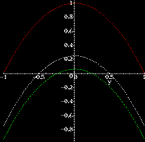
For Example: z=x²-y² can be modeled in three dimensional space, but personally I find it difficult to sketch! In the section on critical points a picture of a plot of this function can be found as an example of a saddle point. But by alternately setting x=1 (red), x=0.5 (white), and x=0.25 (green), we can take slices of z=x²-y² (each one a plane parallel to the z-y plane) and see different partial functions. We can get a further idea of the behavior of the function by considering that the same curves are obtained for x=-1, -0.5 and -0.25.

Food For Thought: How do partial functions compare to level curves and level surfaces? If the function f is a continuous function, does the level set or surface have to be continuous? What about partial functions?

All of this helps us to get to our main topic, that is, partial differentiation. We know how to take the derivative of a single-variable function. What about the derivative of a multi-variable function? What does that even mean? Partial Derivatives are the beginning of an answer to that question.

A partial derivative is the rate of change of a multi-variable function when we allow only one of the variables to change. Specifically, we differentiate with respect to only one variable, regarding all others as constants (now we see the relation to partial functions!). Which essentially means if you know how to take a derivative, you know how to take a partial derivative.

A partial derivative of a function f with respect to a variable x, say z=f(x,y₁,y₂,...y_n) (where the y_i's are other independent variables) is commonly denoted in the following ways:

(referred to as ``partial z, partial x'')

(referred to as ``partial f, partial x'' )

Note that this is not the usual derivative ``d'' . The funny ``d'' symbol in the notation is called ``roundback d'', ``curly d'' or ``del d'' (to distinguish from ``delta d''; the symbol is actually a ``lowercase Greek `delta' '').

The next set of notations for partial derivatives is much more compact and especially used when you are writing down something that uses lots of partial derivatives, especially if they are all different kinds:

(referred to as ``partial z, partial x'')

(referred to as ``partial f, partial x'')

(referred to as ``partial f, partial x'')

Any of the above is equivalent to the limit

.

The actual calculations of partial derivatives for most functions is very easy! Treat every indpendent variable except the one we are interested in as if it were a constant and apply the familiar rules!

Example:

Second Partial Derivatives

For the same reasons, in the case of the expression,

Below are examples of pure second partial derivatives:

Example:

• f_x=ye^xy + ycosx
• f_xy=xye^xy + cosx
• f_y=xe^xy + sinx
• f_yx=xye^xy + cosx

In this example f_xy=f_yx. Is this true in general? Most of the time and in most examples that you will probably ever see, yes. More precisely, if

• both f_xy and f_yx exist for all points near (x₀,y₀)
• and are continuous at (x₀,y₀),

Partial Derivatives of higher order are defined in the obvious way. And as long as suitable continuity exists, it is immaterial in what order a sequence of partial differentiation is carried out.