XCrySDen can
display properties such as charge densities, molecular
orbitals, or any other 2D or 3D scalar field as
isosurface or contours. This means, that a uniform 2D
or 3D grid of points (containing the field
values)---the grid does not need to be
orthogonal---should be provided. Such grids are called
Data Grids by
XCrySDen. In order to
display the isosurfaces/contours, the scalar field data
should be written in XSF format.
Here you can find the
corresponding XSF description. The users of CRYSTAL and
WIEN programs can achieve such plots also using the
XCrySDen's
interface for
CRYSTAL and
WIEN.
Once the XSF file is constructed, one should load it
either as xcrysden --xsf my_file.xsf or
via the File-->Open
Structure ...-->Open XSF(Xcrysden Structure
File) menu. Then proceed via the
Tools-->Data
Grid menu. The following window will
appear:
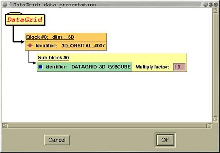
This window plots schematically the
structure of the scalar fields inputs. Namely, XSF file
can contain several scalar fields. In the above example
(i.e. figure of the window) the file contains only one
scalar field. here is an example of window that
corresponds to the file that contains several scalar
fields:
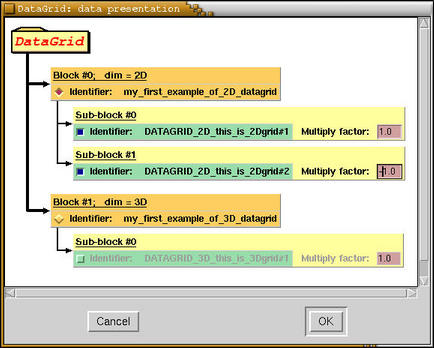
In this example, three scalar fields are
specified (see the three yellow-green rectangles,
designated as sub-blocks). The first two are
two-dimensional, and are mutual compatible, therefore
they are specified within one block (i.e. block #0 on
the figure). The third scalar field is
three-dimensional. Here the user should specify which
scalar field would like to plot. This is achieved by
selecting (i.e. mouse-clicking) one radiobutton on
orange block-rectangles. Then within a block one can
select several scalar fields by mouse-clicking the
corresponding checkbuttons on yellow-green
subblock-rectangles. In above example two scalar fields
are selected (see red checkbuttons on yellow-green
subblock rectangles). A weight (i.e. multiply factor)
for each selected scalar fields should be selected.
Then the resulting scalar fields is calculated as:
Fres(r) =
w(1)*F1(r) +
w(2)*F2(r) + ...,
where w(i) is the weight (i.e. multiply
factor) for i-th selected scalar field.
Once the scalar fields are selected and the weights
are set, press the [OK] button. Then next
window will appear, where various isosurface or
contours parameters can be controlled. Here you can read how to
control the display of the isosurfaces, and here you can get the
description of how to control the display of
contours.


![[Figure]](img/xcrysden-picture-small-new.jpg)