XCrySDen program can be
used as a graphical tool for
WIEN2k, a FP-(L)APW program
package. The following graphical tasks can be performed
by the
XCrySDen program:
- visualization of crystal structures
- graphical selection of k-path inside the
Brillouin zone for spaghetti plots
- visualization of 2D contours/isolines and 3D
isosurfaces (charge density, electrostatic potentail)
- visualization of Fermi surfaces
All these options are accessible either via
File-->Open WIEN2k
... casade menu or via command line
options.
XCrySDen's command line
options intended for WIEN start with the
--wien_ prefix. Currently five different
command line options are supported:
|
Usage:
|
xcrysden [OPTIONS]
                                    [file|filehead|directory]
|
-
xcrysden --wien_struct
                              filehead|file|directory
Corresponding
menu:
File-->Open WIEN2k
...-->Open WIEN2k Struct File
Reads struct file and renders the
crystalline structure.
-
xcrysden --wien_kpath directory
Corresponding menu:
File-->Open WIEN2k
...-->Select k-path Reads
struct file and renders first Brillouin
zone with special k-points. K-path can be
selected interactively by mouse-clicking
appropriate k-points. We must specify
EMIN and EMAX parameters and
total number of k-points along the path. This is
merely an estimation of the total number of
k-points, since XCrySDen tries to
produce a uniform sampling of k-points along the
k-path, therefore don't specify WIEN2k's maximum
allowed number of k-points, as XCrySDen maight
generate few points more.
-
xcrysden --wien_renderdensity
                              directory
Corresponding menu:
File-->Open WIEN2k
...-->Render pre-Calculated
Density Reads struct,
output5 and rho files and renders
crystalline structure and precomputed charge
density.
-
xcrysden --wien_density directory
Corresponding menu:
File-->Open WIEN2k
...-->Calculate & Render
Density First, either 2D or 3D
region for charge density calculation is chosen
grahically by mouse-clicking. Then XCrySDen generates
the in5 file(s), calculates and renders
charge density. The density can be displayed
either as isolines/colorplanes (2D) or an
isosurface (3D).
-
xcrysden --wien_fermisurface
                              directory
Corresponding menu:
File-->Open WIEN2k
...-->Fermi Surface Pops-up a
task window for Fermi surface creation. After
several steps the Fermi surface is hopefully
drawn as 3D isosurface. This feature is
EXPERIMENTAL, please be careful !!! So far it was
tested on a few spin non-polarised and
spin-polarized systems. (Currently the shift of
the k-mesh is not allowed.)
|
LEGEND:
|
directory
|
name of the case directory
|
filehead
|
name of the struct file without
.struct extension
|
filename
|
name of the struct file
|
This option is available via
File-->Open WIEN2k ...-->Select
k-path menu or as
--wien_struct command line option. There
is nothing special for this option. Displaying the
crystal structure from WIEN
struct file is
alike displaying the structure from other supported
formats. The decription of various available
XCrySDen
options for the visualization of crystal structures can
be found in the following documents:
Short Introduction to XCrySDen,
Description of XCrySDen main window and
menus, and
HOWTO: Modify
Menu.
This option is available via
File-->Open WIEN2k ...-->Select
k-path menu or as
xcrysden
                        --wien_kpath directory
command line option. A
special window pops-up where we select a k-path inside
the Brillouin zone (BZ).
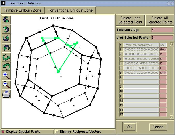
In above window we see two tabs entitled:
(i)
Primitive Brillouin Zone and (ii)
Conventional Brillouin zone. The latter is
provided only for informational purpose, namely, to see
the shape of the BZ tessellated according to the
conventional set of reciprocal vectors. Hence for real
applications we stick to
Primitive Brillouin
Zone and select a k-path by mouse-clicking a
special k-points. The BZ can be rotated by holding-down
left mouse button and dragging the mouse.
For a few Bravais lattice types, several common
k-points will be labelled automatically (thanks to
Peter Blaha), such as GAMMA, X, W, K, L points for
the fcc lattice. The automatic k-point labbeling
currently supports the following Bravais lattice
types:
- primitive cubic
- fcc
- bcc
- primitive tetragonal
- body centered tetragonal
- primitive orthorhomobic
When we are done with the k-points selection the
[OK] button should be pressed and a new window
will appear.
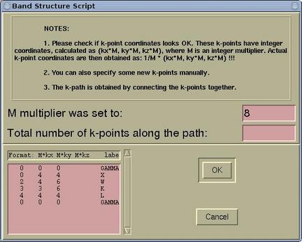
Here we must specify the total number of
k-points along the path. This is merely an estimation
of the total number of k-points. The precise number of
k-points is determined by
XCrySDen in such a way
that the density of k-points is as uniform as possible
for all k-line segments. After pressing the
[OK]
button the file-browser will appear and we can save the
.klist file for spaghetti plot.
This option is available via the
File-->Open WIEN2k
...-->Render pre-Calculated Density
menu or as
xcrysden --wien_renderdensity
                        directory
command line option.
XCrySDen reads the
struct,
output5 and
rho files and
renders crystalline structure and precomputed charge
density as contours or colorplane.
Here you can read how to
control various parameters for contour and colorplane
display.
This option is available via the
File-->Open WIEN2k
...-->Calculate & Render Density
or as
xcrysden --wien_density directory
command line option. First
XCrySDen will ask
whether we want to compute the charge density (or some
other property) in 2D or 3D region:
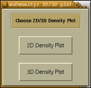
Now we will have to select a region of
space where the charge density will be calculated.
Depending on our choice this will be either 2D or 3D
region.
Here you can
read how to select a 2D region, and below you can read
how to select a 3D region.
The following window is devoted to the selection
of the 3D region of space.
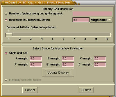
Here is the description of widgets on
above window.
|
[Grid Resolution]
|
You can find the description of this items
here
|
|
[Interpolation]
|
There is a possibility of interpolating a
grid by tri-cubic spline interpolation. At
this stage I would suggest to specify no
interpolation (degree=1), as it will be
possible to do that later.
|
|
[Space Selection]
|
By default the space comprised by the whole
unit cell is selected. Then we have the
possibility to specify the margins. Here you can find
the description about margins.
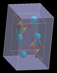
Important: Only after we press the
[Update button] the currently selected
space will be rendered as transparent box. On
the figure below we see the unit-cell space
selection with the
A=B=C=A*=B*=C*=0.2 margins.
|
There are two buttons on the bottom of
3D Map - Grid Specification
window. The function of these buttons is the following:
|
[Cancel]
|
Cancels the process and closes the window
|
|
[Submit]
|
Submits the calculation to the WIEN program.
But before that a special window pop-sup,
where we specify various WIEN related flags.
( Read more ...).
|
The wollowing window is devoted to the selection
of the 2D region of space.
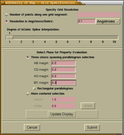
At the top of the window we specify the
grid resolution and an interpolation setting. (
Read more ...). The
second part (label
Select Plane for Property
Evaluation) of the
2D Map - Grid
Specification window is devoted to the selection
of 2D region of space. We can do that via two different
procedures, which are chosen by pressing the
corresponding radiobutton, that is either
[Three-atoms spanning parallelogram selection]
or
[Atom centered selection].
Here you can find
description of these graphical procedures. Two button
are located at the bottom of
2D Map - Grid Specification
window. The description of their function can be found
here.
In the foolowing window the WIEN flags for charge
density calculation are entered:
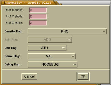
These flags are the same for 2D and 3D
charge density calculation, simply because the latter
calculation in composed of several 2D slice
calculation. For the meaning of this flags you should
refer to WIEN manual.
After we have done all above steps then the
controlling window for either contour or isosurface
display appears, depending on the 2D or 3D choice.
Here you can find
description for the contour display, and
here for isosurface display.
This is a new option and was not yet tested
extensively, please be careful!!! It is available via
File-->Open WIEN2k
...-->Fermi Surface menu or as
xcrysden --wien_fermisurface directory
command line option. First a task window for Fermi
surface creation Pops-up.
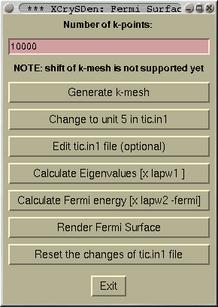
This window style is closely similar to
that of
Wien in a Box, hence it is hopefully
self-explanatory. After series of task (pressing
buttons from top to bottom) are performed, one finally
arives to
[Render Fermi Surface button]. Upon
pressing the button the value of Fermi energy will be
queried. After that two windows will appear:
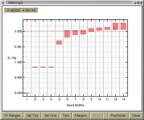
The upper window displays the band-widths.
The Fermi level is also indicated by red horizontal
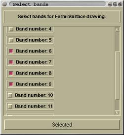
line at 0.66 Ry. The purpose of the bottom window is
the selection of the bands for which the corresponding
part of Fermi surface will be drawn. Usually, one
selects the bands that cross the Fermi level. When the
bands are selected proceed by pressing the button
[Selected]. In a while the Fermi surface of the
first selected band will be displayed in a viewer
window. Actually, the viewer is composed from notebook,
holding the Fermi surfaces of all the bands in separate
pages.
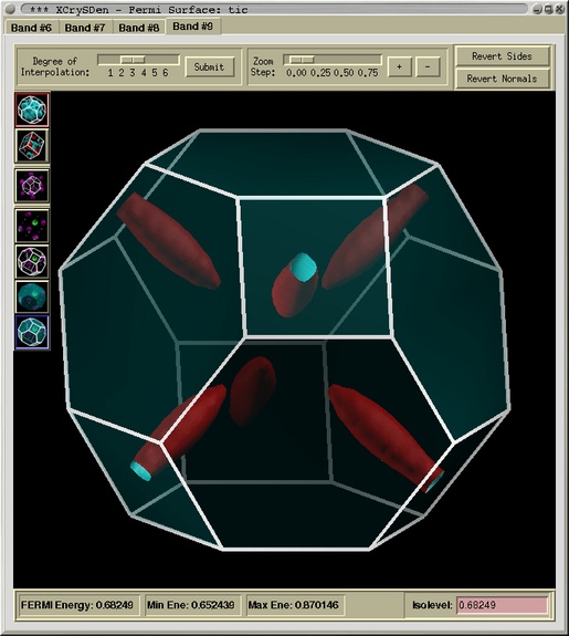
Fermi surface corresponding to the 9th band of
TiC (i.e. the 4th band that crosses the Fermi
level)
Here you can get
more information about the Fermi surface Viewer ...


![[Figure]](img/xcrysden-picture-small-new.jpg)