Complex networks and collective behavior in nature

What is surprising about scale-free networks?

The scale-free network is surprising because was not expected. In nature there are different random processes that generate Poisson distributions (e.g. radioactive decay) or exponential distributions (e. g. electronic component's lifetime), but there are very few precesses that generate scale-free distributions. In fact the work of Erdos and Renyi showed that networks that are growth by randomly adding new nodes and connections have Poisson or exponential topologies. That is the paradox, networks like WWW or the sexual partners network are growth randomly adding new nodes and new connections along time. Then, how is it possible that these neworks that were growth randomly do not have either Poisson or exponential topologies as Erdos and Renyi predicted?.

As we shown in the previous page, the Poisson topology is very different from the scale-free topology. In Poisson structures, the nodes have in average the same number of connections, whereas the most important characteristic in scale-free networks is its high heterogeneity, there are nodes with very few connections, and nodes that are extremly connected. The later are known as hubs. Is still completely unknown what are the processes that lead formation of scale-free networks, however there have been advances in the comprenhension of these networks. In the following sections we will shown some of teh mathematical formalisim to study the growth of networks.

Erdos-Renyi networks (Poisson topology)

Lets imagine a set of $N$ buttons randomly distributed on a table and initially unconnected. At time t = 0, we randomly pick a pair of buttons and we tie those together with thread. After connect them, we release again the buttons on the table an again we pick two buttons. We can select buttons that are connected with others, but we discard the pair if we selected one that has been selected before. Lets repeat the operation $M$ times. At the end of this process, we will end with $M$ joints between $M$ different pairs, generating a network of buttons. Intuitively we know that if $M$ is small compared to $N$ , then the resultant network will be composed by many small islands. In each island the buttons will be attached by threads, but there will be disconnected from other islands. However if $M$ is as large as $N$ , we will end with almost all the buttons joined to each other.

After having selected $M$ pairs in a set of $N$ buttons, what will be the degree of connections, $P(k)$ in the resultant network?. As we will see in a moment, the resultant network has a Poisson distribution. Before to proof that, it is important to mention that for a long time people thought that this mechanism of network growing in which pairs are randomly joined was the suitable model to describe social networks like friendship networks or sexual partners networks. It was natural to think networks like those that are growth by random meetings between people in a society could be described by the mechanism just shown. It was natural but it was incorrect.

Let calculate the probability, $P(k)$ , for our buttons network. To start, lets consider the total number of pairs $N_{p}$ that can be formed from a set of $N$ buttons is:

$N_{p} = \frac{1}{2}N\left (N-1 \right )$

We selected $M$ buttons pairs, so the probability $p_{e}$ of a randomly selected pair of being attached is:

$p_e=\frac{M}{N_{p}}=\frac{2M}{N\left (N-1 \right )}$

Now lets focus in one particular node, $v_{j}$ , that was randomly chosen. The total number of pairs that could contain $v_{j}$ , is $N-1$ , because we could have attached $v_{j}$ with the remaining $N-1$ nodes. However within the $M$ selected pairs, we didn't select necessarily $v_{j}$ all the possible times. Lets say that $v_{j}$ was selected $k$ times in the $M$ pairs. Then, the probability of $v_{j}$ of being in $k$ of the $N-1$ possible pairs is

$P(k) = \binom{N-1}{k}\left ( p_e \right )^{k}\left ( 1-p_e \right )^{N-1}$ The last expression is know as the binomial distribution for finite N and M. If we consider a giant network and we take the limit $N\to \infty$ and $M\to \infty$ such that $z$ remains finite, then the distribution turns into the following expression, which is the Poisson distribution.
$P(k)=e^{-z}\frac{z^{k}}{k!} \qquad ; \qquad z = \frac{2M}{N}$

Network growth

In the description above presented we assumed that we had a fixed population $N$ of nodes and a fixed number $M$ of conecctions randomly added to built the network. However, networks are not fixed systems. The complex networks evolve and they grow on time by adding nodes and connections. For example, in 1969, internet network was composed only by two computers, one in the University of California at Los Angeles (UCLA) and the other in the Stanford Research Institute (SRI). In 2000 that network inlcuded 170 countries and more than 300 millions of people.

As the last example just showed, our model needs to take in count the possibility of adding new nodes and new conecctions as well as the elimination of previously present connections and nodes. In the simplest model of network growth, que can add a new node in each time step. This new node can be connected with any previously present node. Then, the probability of each node of being selected is $\Pi (k_i,t)$ , where $k_{i}$ is the i-th node connectivity at time t.

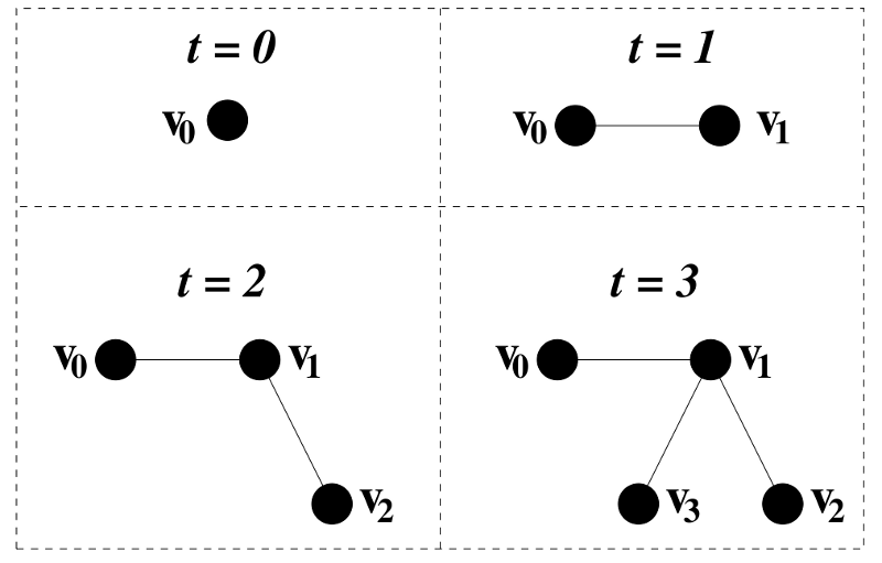
The growth process starts with a unique initial node $v_{0}$ at time $t=0}$ . At $t=1}$ we add a new node $v_{1}$ , that will be connected to the only existing node $v_{0}$ with probability 1. At time $t=2}$ we add a new node $v_{2}$ that can be connected to either $v_{0}$ or $v_{1}$ with the same probability 0.5. At this point, the nodes $v_{0}$ , $v_{1}$ and $v_{2}$ no longer have the same connectivity. Any of these three will have two connections, whereas the other two will have just one connection. At time $t=3}$ we add a new node $v_{3}$ that can be connected to either $v_{0}$ , $v_{1}$ or > $v_{2}$ with a probability that will be a function of their connectivities $k_{0}$ , $k_{1}$ and $k_{2}$ . Following htis protocol, at time $t+1}$ we add the node $v_{t+1}$ that will be connected to any of the existing nodes, $v_{0}$ , $v_{1}$ ... $v_{t}$ , the later will be selected with a probability $\Pi (k_i,t)$ , where $k_{i}$ is the i-th node connectivity at time $t}$ .

Network growth At time $t=0}$ there is just one node $v_{0}$ . in each subsequent step, we add a new node that will be connected to any of the previous existing nodes with a probability $\Pi (k_i,t)$ that depends on the connectivity $k_{i}$ of the i-th node at time $t}$

Lets denote as $P(k,t)$ to the probability that at time $t}$ an arbitrary node within the network had $k}$ connections. It is clear that the probability depends on time. However, we expect that if we continue adding nodes for a long enough time, we will reach a point in which $P(k,t)$ no longer depends on time. Such as that point is known as stationary state. It is important to remark that the network keeps growing as we add more nodes, but the connections degree (or connections distribution ) $P(k,t)$ , is the one that reaches a state in which $P(k,t+1) = P(k,t) = P(k)$ , the connection distribution no longer depends on time.

There are different approaches to calculate the connection distribution $P(k,t)$ , but the mathematical formulation of any of those is out of the scope of this introductory page. Instead we will show just the results for the master equation approach.

The master equation approach includes the two following contributions to calculate the temporal evolution of the connection distribution, $P(i,k,t)$ , associated to the node $v_{i}$ .

At time $t}$ , the node $v_{i}$ had $k-1$ connections and was selected (with probability $\Pi (k-1,t)$ ) to be connected with the new added node. Furthermore, at time $t+1}$ , the node $v_{i}$ will have $k$ connections.
At time $t}$ , the node $v_{i}$ already had $k$ connections and was not selected (with probability $1-\Pi (k,t)$ ) to be connected with the new added node. Furthermore, at time $t+1}$ , the node $v_{i}$ will still have $k$ connections.

We should note that in order to be able to solve the time evolution of $P(i,k,t)}$ we need to know the explicit form of $\Pi (k,t)$ , which is the probability of an existing node with conectivity $k$ of being selected to form a connection with the new node that is added at time $t$ . As we will see in the following section differents expressions for $\Pi (k,t)$ led to different topologies.

Back Next